
Distributed Storage Patterns For Model Checkpoints
If your cluster fails every 4 to 22 hours, checkpoint layout can decide whether you lose minutes of work or a huge chunk of a training run. My take is simple: use shard-based checkpoints for most large training jobs, use local staging when you checkpoint often and need training to keep moving, use larger consolidated files when portability matters more than save speed, and avoid many tiny per-rank files once metadata load starts to bite.
Here’s the short version in plain English:
- Many small checkpoints give high parallel writes, but they can crush filesystem metadata and inode limits.
- Fewer large files cut namespace pressure, but restore and write time become bound by moving one huge file, and one bad file can kill the whole snapshot.
- Shard-based layouts are often the best middle ground for large-scale training: parallel I/O, lower metadata stress, and good restart behavior.
- Staged local-to-shared checkpointing keeps GPUs from waiting on shared storage by writing to local RAM or NVMe first, then copying out later.
- The main things to judge are checkpoint frequency, model size, GPU count, restart goals, and storage backend.
A few numbers show why this matters:
- Cluster failures can slow training by up to 43%
- BLOOM 176B uses a 329 GiB checkpoint split into 72 shards
- One staged setup cut checkpoint blocking from 2 minutes to 0.2 seconds
- Parallel decompression reached 3.76 GiB/s
Lightning Talk: In-Cluster Distributed Checkpointing: Optimizing Training... - G. Kroiz & S. Mishra
sbb-itb-903b5f2
Quick Comparison
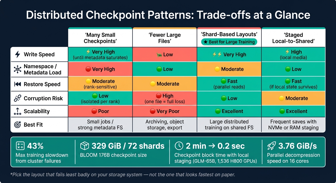
Distributed Checkpoint Patterns: Trade-offs at a Glance
| Pattern | Write Behavior | Main Pain Point | Restart Profile | Best Fit |
|---|---|---|---|---|
| Many Small Checkpoints | Very parallel | Metadata and inode pressure | Good if rank mapping stays aligned | Smaller jobs or filesystems with strong metadata handling |
| Fewer Large Files | Fewer writes, larger transfers | Single-file bandwidth and corruption risk | Moderate | Archiving, export, object storage |
| Shard-Based Layouts | Parallel shard writes | Shard tracking and commit logic | Strong parallel restore | Large distributed training on shared filesystems |
| Staged Local-to-Shared | Local write first, shared copy later | Local space limits and extra state tracking | Very fast if local state survives | Frequent checkpoints with NVMe or RAM staging |
If I had to reduce the whole topic to one rule, it would be this: pick the layout that fails least badly on your storage system, not the one that looks fastest on paper. That means watching free space, inode counts, commit status, and restore behavior just as closely as raw write speed.
1. Many Small Checkpoints
Each GPU rank writes its own shard on its own. That keeps writes fully parallel, which is great for speed. The flip side is simple: the file system has to deal with a lot more pressure.
Write Path Efficiency
On 128 A100 GPUs, IBM and Meta's LlamaT run cut checkpoint time by an order of magnitude with PyTorch FSDP distributed checkpointing. That kind of setup is fast because every rank writes at the same time.
But there’s a catch. The same parallel write pattern that helps throughput also drives up metadata traffic.
Metadata and Namespace Overhead
This is the tradeoff. When hundreds of GPU ranks each write their own file at once, the file system has to process thousands of metadata operations in parallel. Even if raw I/O bandwidth is sitting there ready to go, distributed file system metadata servers can still become the choke point.
Checkpoint more often, and that pressure stacks up fast. If the file system can handle it, though, the same layout can also make restores just as fast.
Restore and Recovery Speed
Recovery follows the same pattern as writing: each rank reads back its own shard in parallel. In BG-LMC, decompression reaches 3.76 GiB/s, compared with 2.78 GiB/s on compression. In plain English, recovery usually moves faster than writing.
That edge can vanish if storage capacity or inode limits become the thing holding you back.
Backend Fit and Operational Risk
The biggest day-to-day risk is silent disk exhaustion. In the same LlamaT run, disk space filled at 1.5T tokens. Training kept going, but checkpointing failed, so the last recoverable state stayed at 1.5T tokens.
Many-small-checkpoint layouts can also run into inode limits, which is a different ceiling from raw disk capacity. A system can have free space left and still fail because it has run out of inodes. That’s why it’s smart to watch both capacity and inode count throughout training.
2. Fewer Large Checkpoint Files
When lots of small checkpoints swamp metadata, using fewer, larger files flips the bottleneck. Instead of stressing metadata services, checkpointing starts to lean hard on sequential throughput and network bandwidth. In this setup, a single checkpoint can grow to 329 GiB.
This layout trims metadata traffic, keeps inode use down, and cuts the constant open/close churn that distributed file systems like Lustre or CephFS have to deal with. That takes pressure off the file system. But restore time still comes down to one plain fact: how fast you can move that big chunk of data.
Restore is still bandwidth-bound, even if decompression is fast. In one case, decompression reached 3.76 GiB/s on 16 cores. So the CPU side may keep up, but the file still has to travel across storage and network links.
There’s also a trade-off with fault isolation. With smaller shards, one bad file usually hurts only one rank’s state. With one large file, corruption can wipe out the entire checkpoint.
That risk shows up during writes too. A large checkpoint file has to finish writing before the next checkpoint interval. If the write runs long or the file ends up corrupted, the whole snapshot can fail.
At that point, teams often swing back toward shard-based layouts. Once a single file gets too big to move well, splitting the checkpoint across parallel writers becomes the more workable path.
3. Shard-Based Checkpoint Layouts
Shard-based layouts sit in the middle between tiny-file setups that hammer metadata services and giant checkpoint files that put too much strain on bandwidth. Each training rank writes its own part of the model state to a separate shard file. So you get a small set of parallel writers instead of a flood of tiny file operations. That keeps write parallelism in place without sliding back into the metadata churn that comes with many small files.
Write Path Efficiency
In PyTorch FSDP, distributed checkpointing moves GPU state into host RAM first, then writes shard files to shared storage asynchronously. That cuts GPU idle time during checkpoint saves. The main reason is simple: each rank writes its own local shard instead of funneling everything through one place.
Metadata Overhead
Shard counts stay low enough to avoid metadata storms, while still letting ranks write in parallel. BLOOM 176B is a good example. Its checkpoint is 329 GiB and is split into 72 shards across 48 nodes and 384 GPUs. Compression can help too. The Language Model Compressor (LMC) reaches 2.78 GiB/s on 16 cores.
Restore and Recovery Speed
The same layout that helps on writes also helps on reload. Each rank reads back only its own shard, so restore work spreads out in parallel. No single rank has to sit around waiting for another one to finish first.
Storage Risk
There is still a catch. Shard-based layouts fail when storage space runs out. If the storage system fills up, checkpoint writes can stop silently while training keeps going. When that happens, the last usable recovery point is stuck at whatever step was saved before capacity was exhausted.
4. Staged Local-to-Shared Checkpointing
This pattern writes checkpoint data to local RAM or NVMe first, then sends it to shared storage in the background. The big shift is simple: the training job no longer waits on shared storage before moving on. The slow part drops out of the critical path, and local bandwidth takes over.
Write Path Efficiency
Once the state lands in local memory, training can continue while the checkpoint is copied to shared storage. That changes the timing in a big way.
A 16-core parallel implementation of LMC can hit 2.78 GiB/s during staging, which cuts down the amount of data that later needs to be written to shared storage.
Metadata and Namespace Overhead
This pattern isn't free. Staged checkpointing adds metadata for segment counts, sizes, and deltas. If you also use incremental snapshotting, XOR deltas between training steps add one more layer of state to track.
That extra bookkeeping only pays off if the local state sticks around long enough to support a restart.
Restore and Recovery Speed
Restore speed depends a lot on what survives the fault. If host memory is still there, recovery is the best-case scenario. About 75% of training faults fall into that bucket, so restart can be almost instant.
One GLM-65B training run on 1,536 H800 GPUs shows how much this can matter. Staged checkpointing reduced training block time from 2 minutes to 0.2 seconds per checkpoint. That made it possible to move from checkpointing every 250 steps to every 10 steps. If a node fails and local memory is gone, though, restore drops back to minutes.
Backend Fit and Operational Risk
The hardware setup makes or breaks this pattern. Local staging works best with NVMe SSDs or RAM disks. In plain terms, you need fast local media and enough room to absorb checkpoint bursts.
Watch local capacity closely. If that space fills up, new checkpoints can fail even if training keeps running.
Pros and Cons by Storage Pattern
Each pattern makes a different trade-off between write speed, metadata load, restore speed, and day-to-day ops work. The table gives you the quick view. The notes right after it zoom in on the main thing that tends to break first.
| Many Small Checkpoints | Fewer Large Files | Shard-Based Layouts | Local Staging | |
|---|---|---|---|---|
| Namespace Load | Very high | Low | Moderate - shard mapping required | Low |
| Write Speed | High - until metadata saturates | Low (consolidation bottleneck) | Very high (distributed) | High (local media speed) |
| Restore Speed | Slower if rank placement changes | Moderate | Fast (parallel reads per rank) | Fast if local state survives |
| Metadata Overhead | Very high at filesystem level | Low | Moderate (shard-to-rank mapping) | Low |
| Operational Complexity | Low | Low to moderate | High (requires FSDP/DCP) | High (async management) |
| Scalability | Poor | Very poor | Excellent | Excellent |
The short version: no layout wins on every axis.
Many small checkpoints give you the best raw parallelism, but they hit metadata pressure hard. The setup is simple, which is nice, yet namespace load becomes the thing that holds you back as rank count climbs.
Fewer large files keep the namespace simple, but write throughput takes a hit. Shards have to be merged before writeout, and one corrupted file can wipe out the whole checkpoint.
Shard-based layouts hit the best middle ground for throughput and metadata load. Each rank writes and reloads only its own shard, so writes and restores don't get funneled through one chokepoint. At that stage, the main limit is bookkeeping rather than throughput.
Local staging keeps GPU idle time low, but it leans heavily on local storage. It works well when spill space is there, and gets fragile fast when it isn't.
How to Choose Based on Training and Storage Constraints
Use the tradeoffs above to match your checkpoint layout to the job and the storage system behind it. Four things matter most: checkpoint frequency, model size, worker count, and restart target. Get this wrong, and storage becomes the choke point.
Checkpoint frequency and model size come first. If you save often and the model state is large, checkpointing creates burst writes. That can slow training if shared storage can’t keep up. In that case, use staged local-to-shared checkpointing so writes land on local storage first and move to shared storage after. If saves happen less often, shard-based layouts can usually handle the load without the extra staging step.
Worker count is the next filter. As GPU count grows, layouts with lots of small files tend to hit metadata limits before anything else. That’s where shard-based layouts make more sense. Use HSDP when the model fits within a node and inter-node traffic is the main limit.
Storage backend often settles the choice:
| Storage Backend | Best Pattern | Why |
|---|---|---|
| Node-local NVMe | Staged Local-to-Shared | Absorbs write bursts; very high throughput |
| Distributed File System | Shard-Based Layouts | Avoids metadata saturation across workers |
| Object Storage | Fewer Large Files | High metadata latency penalizes small-file writes |
Restart time targets also matter. If you need short restart times, lean toward shard-based layouts and fast decompression. Parallel decompression can reach 3.76 GiB/s on a 16-core system, so layout choices have a direct effect when restart speed is tight.
That makes restart time the last filter before you get into implementation details.
Implementation Details That Affect the Outcome
A storage pattern only works if commit, validation, and reload are handled the right way. Those three pieces decide whether a checkpoint can be restored or whether it just looks saved.
Manifest design is where restore logic begins. If you're working with multi-file checkpoints, keep a manifest or completion record that points to the latest valid checkpoint and lists its files. That's the line between a complete snapshot and a half-finished write.
Distributed and centralized write paths need different guardrails. For single-file writes, use rank 0 so multiple processes don't fight over the same path. For distributed layouts, use sharded writes. Once that path is set, the next problem is the one that tends to slip by: silent failure.
Silent failures are the real danger.
Training can keep going even after writes fail. That's why a missed commit should trigger an alert before the next save runs. Check free space, and confirm every checkpoint commit before moving on. If storage runs out and nobody notices, checkpointing doesn't just stop for a bit - it wipes out the recovery value of every step that comes after it.
After commit checks, validation is the last safeguard. Don't rely on file-level SHA256 for PyTorch zip checkpoints. Container metadata can change even when the tensor data stays the same. Check at the tensor level instead, or use tooling that ignores container metadata. If node count or topology changes, convert shards before re-sharding for the target layout.
Conclusion
There’s no single checkpoint pattern that works best in every case. The right pick depends on three things: how often you save, how fast you need to restart, and how much storage headroom you have.
Shard-based layouts make the most sense for active training with frequent saves. They split write pressure across files and help ranks load in parallel, which cuts restart friction. Consolidated files make more sense after training, when moving, sharing, or archiving the model matters more. They’re simpler to handle and easier to ship around.
Use this summary:
| Scenario | Recommended Pattern | Key Reason |
|---|---|---|
| Frequent saves during training | Shard-Based Layouts (FSDP/DCP) | Spreads write bursts and supports parallel reads across ranks |
| Infrequent large snapshots | Fewer Large Consolidated Files | Simplifies portability for evaluation or deployment |
| Fastest restart target | Per-rank shards | Each rank reloads its own state directly |
| Metadata-constrained distributed FS | Fewer Large Files (Consolidated) | Reduces file entries and avoids metadata server saturation |
| Small-to-mid scale models | HSDP | Reduces inter-node traffic |
No matter which pattern you use, the day-to-day basics don’t change: check checkpoint integrity from time to time during long-running jobs, and watch disk capacity before it turns into an outage. The layout sets the upper bound. Validation and capacity checks decide whether checkpointing holds up when you need it.
FAQs
Which checkpoint layout should I choose first?
Start with your model size and parallelism plan. For small to mid-sized models, DDP with a rank 0 master-process setup is often enough. It’s simple, easy to run, and usually gets the job done.
If your model is too large to fit within GPU memory limits, switch to a sharded setup like FSDP. That spreads model states across devices instead of trying to cram everything onto each GPU.
No matter which layout you pick, put asynchronous checkpointing near the top of your list. Write checkpoints to local NVMe SSDs first, then move them to persistent storage. That helps keep training from slowing to a crawl every time you save state.
When does local staging outperform shard-based checkpoints?
Local staging beats shard-based checkpointing when the main goal is simple: keep GPUs from sitting idle and write checkpoints as fast as possible.
Here’s why. Instead of sending checkpoint data straight to shared storage, local staging writes it to nearby NVMe SSDs first. Those drives can handle about 50–200 GB/s, which means training can start again much sooner while the data is copied to persistent storage in the background.
That matters a lot for high-volume jobs and ultra-low-latency setups. By sidestepping the immediate network traffic spike from many machines writing to shared storage at the same time, local staging cuts one of the biggest slowdowns during checkpointing.
How do I prevent silent checkpoint failures?
Prevent silent checkpoint failures by watching both your storage setup and the training job itself. One of the most common issues is simple: the disk fills up. Training may keep running, but the checkpoint ends up partial or never gets written at all.
It also helps to keep an eye on storage throughput and latency. If writes slow to a crawl, checkpoint saves can fail or stall without much warning. In distributed training, save checkpoints only from the primary rank, rank 0, so multiple workers don't step on each other.
Use clear file names, and set up automatic retention so older files get cleaned up on schedule. That way, recent valid checkpoints stay on hand instead of getting buried, overwritten, or lost when you need them most.