5 Partitioning Methods for Multi-GPU Training
Training massive AI models across multiple GPUs is essential for handling their memory and computational demands. From GPT-3 to LLaMA, these models are too large for a single GPU, even high-end ones like NVIDIA's A100. To address this, various partitioning methods distribute workloads efficiently across GPUs. Here's a breakdown of the five most effective strategies:
- Data Parallelism: Duplicates the model on each GPU, splitting training data across devices. Best for models that fit on a single GPU but require faster training.
- Model Parallelism: Splits the model itself across GPUs, ideal for architectures too large for one GPU.
- Pipeline Parallelism: Assigns sequential model layers to GPUs, reducing memory needs and improving scalability for deep models.
- Sharded Data Parallelism: Distributes model states (parameters, gradients, optimizer states) across GPUs to reduce memory duplication.
- Fully Sharded Data Parallelism (FSDP): Optimizes memory further by completely sharding all model components, enabling efficient training of trillion-parameter models.
Each method balances memory efficiency, communication overhead, and scalability differently. The right choice depends on your model size, hardware, and training goals.
Quick Comparison:
| Method | Memory Efficiency | Communication Overhead | Scalability | Best Use Cases |
|---|---|---|---|---|
| Data Parallelism | Low (model replicated) | Moderate (All-Reduce) | Limited to single-GPU memory | Small models or high-throughput training |
| Model Parallelism | High (model split) | High (frequent sync) | Moderate (8-16 GPUs) | Large models exceeding single-GPU memory |
| Pipeline Parallelism | High (layers split) | Medium (pipeline bubbles) | Good for deep models | Deep models with sequential architectures |
| Sharded Data Parallelism | High (states sharded) | Moderate (frequent sync) | Excellent for large models | Models >500M parameters |
| Fully Sharded Data Parallelism | Very High (all sharded) | High (intensive sync) | Scales to trillions of params | Trillion-parameter models, memory-limited setups |
These methods enable training of ever-larger models by addressing memory and communication challenges. Whether you're working with a small transformer or a trillion-parameter LLM, there's a strategy to fit your needs.
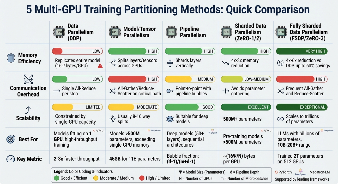
Multi-GPU Training Methods Comparison: Memory Efficiency, Communication Overhead, and Scalability
Multi GPU Fine tuning with DDP and FSDP
sbb-itb-903b5f2
1. Data Parallelism
Data parallelism is one of the simpler ways to train models across multiple GPUs. Here's how it works: the model is duplicated across all GPUs, and each GPU processes a different chunk of the training data at the same time. Once each GPU computes gradients for its portion of the data, these gradients are averaged across devices using an All-Reduce operation. This ensures all GPUs update their weights in sync. Let's explore how this method impacts memory, scalability, and communication.
Memory Efficiency
Data parallelism can be demanding on memory. Each GPU holds a full copy of the model's parameters, gradients, and optimizer states. For example, training a 1-billion-parameter model with the Adam optimizer in mixed precision could require around 16 GB of VRAM per GPU. This means the entire model must fit within the memory of one GPU. If it doesn’t, techniques like gradient accumulation may be necessary to make it work.
Scalability
When GPUs are linked by fast interconnects like NVLink, data parallelism scales almost linearly. The Ring All-Reduce algorithm plays a key role here, using a constant amount of bandwidth - about 2K bytes per GPU, where K is the size of the gradients - no matter how many GPUs are in the system. That said, scalability is still constrained by the memory capacity of individual GPUs.
Communication Overhead
One of the biggest challenges in data parallelism is synchronizing gradients. After each training step, all GPUs need to share and average their gradients before moving forward. This process can become a bottleneck, especially for large models or when network speeds are slow. PyTorch's DistributedDataParallel (DDP) addresses this by overlapping communication with computation. As the PyTorch documentation explains:
"DDP is recommended because it reduces communication overhead … and scales to more than one machine" (PyTorch Documentation).
This optimization makes DDP a go-to solution for minimizing the communication delays inherent in data parallelism.
Best Use Cases
Data parallelism shines in cases where the model is small enough to fit comfortably on a single GPU but requires faster training or larger batch sizes. It's particularly effective for models like ResNet50 or smaller transformer architectures. To get the best performance, use PyTorch's DistributedDataParallel, which avoids Python's Global Interpreter Lock by leveraging multi-processing. For NVIDIA GPUs, combining DDP with the NCCL backend ensures fast communication between GPUs.
2. Model Parallelism
Model parallelism takes a different approach from data parallelism by dividing the model itself across GPUs rather than creating copies of it. This method is especially useful for models that are too large to fit within a single GPU's memory. As AI researcher Luhui Hu notes:
"Parallelism is a framework strategy to tackle the size of large models or improve training efficiency, and distribution is an infrastructure architecture to scale out."
There are two main ways to split a model in this approach: pipeline parallelism, which assigns layers of the model to different GPUs, and tensor parallelism, which breaks down operations within layers across GPUs. For extremely large models, these methods are often combined with data parallelism in what's known as 3D parallelism. Unlike data parallelism, which duplicates the model across GPUs, model parallelism divides it strategically to handle the demands of massive architectures.
Memory Efficiency
One of the biggest advantages of model parallelism is its ability to work around memory limitations. For example, an 11-billion-parameter model requires approximately 45 GB just for its weights, which is far beyond the capacity of most single GPUs. By distributing the model's parameters, gradients, and optimizer states across multiple GPUs, training such enormous models becomes feasible. Advanced methods like ZeRO-3 have even enabled training models with over 2 trillion parameters on 512 GPUs.
Scalability
While model parallelism can scale to large numbers of GPUs, it isn't as straightforward as data parallelism. Poor implementation can lead to inefficiencies, like GPUs idling while waiting for synchronization - a problem referred to as the "pipeline bubble." This inefficiency can be calculated as approximately (d–1)/(m+d–1), where d is the number of partitions and m is the number of micro-batches.
Tensor parallelism performs best within a single node (usually 8 GPUs or fewer) because it relies on extremely high-bandwidth connections like NVLink. On the other hand, pipeline parallelism is better suited for scaling across multiple nodes. These scalability challenges are heavily influenced by how GPUs communicate during training.
Communication Overhead
Memory constraints are only part of the challenge - efficient communication between GPUs is just as critical. The communication demands differ between tensor and pipeline parallelism. Tensor parallelism requires frequent synchronization within individual layers, which depends on high-speed interconnections between GPUs. Pipeline parallelism, in contrast, involves transferring activations and gradients between stages. While this is less communication-intensive, it can still slow down training. In 2020, OpenAI trained GPT-3 using tensor parallelism within 8-GPU nodes and pipeline parallelism across nodes in a Microsoft Azure AI Supercomputer with over 10,000 GPUs.
Best Use Cases
Model parallelism is particularly useful for models with more than 500 million parameters or those with very deep architectures (50+ layers). It ensures that multi-GPU setups operate efficiently. For example, NVIDIA suggests specific configurations based on model size: LLaMA-3 70B runs on 64 GPUs using a combination of 4-way tensor parallelism, 4-way pipeline parallelism, 2-way context parallelism, and 2-way data parallelism. Meanwhile, DeepSeek-V3 671B utilizes 1,024 GPUs with 2-way tensor parallelism, 16-way pipeline parallelism, and 64-way expert parallelism.
However, if your model can fit on a single GPU, data parallelism is often the simpler and more efficient choice.
3. Pipeline Parallelism
Pipeline parallelism works by splitting a model's layers across multiple GPUs. Each GPU is responsible for the weights of its assigned layers, making this approach ideal for deep neural networks with many sequential layers.
A key component of this method is micro-batching, which divides batches into smaller micro-batches. This allows GPUs to process data concurrently. Scheduling techniques, like PipeDream's 1F1B, further enhance efficiency by starting the backward pass as soon as the final forward pass is complete. This reduces the need for cached activations and lightens the memory load on each GPU.
Memory Efficiency
Consider BLOOM's 175-billion-parameter model, which uses bfloat16 and requires about 350 GB of memory for the weights alone - far exceeding the 80 GB capacity of high-end GPUs. Pipeline parallelism solves this by distributing the layers across multiple devices. When combined with activation checkpointing, memory demands are reduced from O(N) to O(√N), though this comes at the cost of roughly 33% more computation time.
Scalability
Pipeline parallelism is designed to scale efficiently across multiple nodes. Instead of relying on global All-Reduce operations like data parallelism, it uses point-to-point communication between consecutive stages. This minimizes idle GPU time and improves scalability. However, reducing "pipeline bubbles" - periods when GPUs are idle - is crucial for performance. The bubble fraction can be estimated with the formula (d–1)/(m+d–1), where d is the number of pipeline stages and m is the number of micro-batches. In practice, pipeline bubbles become negligible when the number of micro-batches exceeds four times the number of pipeline stages. For example, this approach was key to training GPT-3's 175-billion-parameter model across more than 10,000 GPUs, combining pipeline parallelism between nodes with tensor parallelism within each 8-GPU node.
Best Use Cases
Pipeline parallelism shines in deep models, such as Transformers with dozens of layers, where the architecture naturally splits into sequential stages. To maximize performance, it's crucial to balance the computational load across all pipeline stages. Uneven workloads can lead to inefficiencies, with faster stages waiting for slower ones. For training models with over 100 billion parameters, combining pipeline parallelism with tensor and data parallelism - known as "3D parallelism" - is essential. BLOOM's 175-billion-parameter model, for instance, was trained using 384 NVIDIA A100 GPUs with this combined strategy.
4. Sharded Data Parallelism
Sharded data parallelism (SDP) splits a model's training state across multiple GPUs. Each GPU holds only a unique portion - or shard - of the parameters, gradients, and optimizer states. This eliminates duplicate memory usage, unlike traditional approaches, and significantly improves memory efficiency .
Memory Efficiency
Let’s break it down: A model with Ψ parameters in FP32 using Adam optimizer would typically require 16Ψ bytes per GPU under standard DDP (4 bytes for parameters, 4 for gradients, and 8 for optimizer states). With sharding, this drops to roughly (16Ψ/N) bytes per GPU, where N is the number of GPUs. That’s up to a 63% memory reduction . Take the 7-billion-parameter LLaMA model as an example - its training state demands about 112 GB of VRAM, far exceeding the 80 GB capacity of an NVIDIA A100 GPU. Sharding spreads this load across multiple GPUs, making such large-scale training feasible.
Scalability
Beyond memory savings, SDP opens the door to training models with billions - or even trillions - of parameters. For instance, in 2023, Amazon SageMaker trained a GPT-NEOX-20B model using 2 ml.p4d.24xlarge instances (16 GPUs in total) with a sharded data parallel degree of 16 and a sequence length of 2,048. When training a larger 65-billion-parameter model, they scaled up to 64 instances, combining a sharded data parallel degree of 16 with a tensor parallel degree of 8. This method achieves near-linear throughput scaling, effectively overcoming the memory constraints of individual GPUs.
Communication Overhead
The tradeoff for SDP’s memory efficiency is increased communication overhead. Instead of DDP’s single all-reduce operation, SDP relies on more frequent all-gather and reduce-scatter operations. These are used to fetch parameters on demand during computation and synchronize gradients during the backward pass . To minimize delays, frameworks incorporate prefetching techniques, overlapping communication with computation by fetching the next layer’s shards in the background while processing the current layer. Even with these optimizations, collective operations can still consume about 20% of the forward pass time.
Best Use Cases
SDP shines when a model’s memory needs surpass the capacity of a single GPU. It’s particularly well-suited for training and fine-tuning massive language models like GPT-NEOX or LLaMA. To make the most of it, increase the sharding degree until both the model and batch size fit within the available GPU memory. For transformer-based models, using a transformer_auto_wrap_policy ensures that sharding boundaries align with transformer blocks, improving the overlap of communication and computation. Combining SDP with other techniques like mixed-precision training (FP16 or BF16) or activation checkpointing can further optimize memory usage .
5. Fully Sharded Data Parallelism
Fully Sharded Data Parallelism (FSDP) takes memory optimization to the next level by completely eliminating redundant memory usage. Unlike other sharding techniques that may still duplicate certain components, FSDP ensures that all model elements - parameters, gradients, and optimizer states - are evenly distributed across GPUs. During computation, parameters are gathered when needed and then reshuffled immediately afterward. This approach ensures that only one part of the model, such as a transformer block, is fully loaded into memory at any given time. By refining the principles of sharded data parallelism, FSDP maximizes memory efficiency for large-scale training.
Memory Efficiency
FSDP achieves unparalleled memory reduction in distributed training setups. With N GPUs, memory usage scales linearly, significantly lowering the burden on individual GPUs. This shifts the memory limitations from a single GPU to the total memory available across the entire GPU cluster. For models that still push the boundaries of the cluster's memory, FSDP offers CPU offloading, temporarily moving inactive parameters to CPU RAM. This method has enabled training of models with over 40 billion parameters and scaling up to an impressive 2 trillion parameters using 512 GPUs, as demonstrated by DeepSpeed.
Scalability
"FSDP is the recommended strategy when a model's memory requirements exceed the capacity of a single GPU." - Uplatz Blog
FSDP shines when pre-training massive models with 10 billion to 20 billion or more parameters. Its scalability allows efficient training across a wide range of large models, making it a top choice for handling such enormous workloads.
Communication Overhead
While FSDP offers unmatched memory efficiency, it comes with a tradeoff: increased communication demands. Unlike Distributed Data Parallel's single all-reduce operation, FSDP requires frequent all-gather operations to reconstruct parameters for forward passes and reduce-scatter operations to synchronize gradients during backward passes. This makes FSDP highly dependent on network performance. On slower interconnects, communication delays can even surpass computation time. To address this, prefetching can be used to overlap the all-gather operations of the next module with the current module's computation. For multi-node setups, the HYBRID_SHARD strategy - fully sharding within nodes (using fast NVLink) while replicating across nodes - can effectively reduce slower inter-node communication.
Best Use Cases
FSDP is ideal for training and fine-tuning transformer-based models that exceed the memory capacity of a single GPU. The transformer_auto_wrap_policy is particularly helpful, as it aligns sharding boundaries with transformer blocks, optimizing communication and computation overlap. For pre-training models in the 10B to 20B+ parameter range, simply scale the number of GPUs until the model fits comfortably. For fine-tuning on smaller hardware setups, CPU offloading enables training, albeit at a slower pace. Combining FSDP with techniques like mixed-precision training (using bfloat16 for parameters and float32 for gradients) and activation checkpointing can further stretch memory efficiency to its limits.
Method Comparison Table
Choosing the right partitioning method depends on factors like memory availability, network speed, and model size. The table below serves as a quick reference to help you weigh these factors and make an informed decision.
| Method | Memory Efficiency | Communication Overhead | Scalability | Implementation Frameworks | Typical Use Cases |
|---|---|---|---|---|---|
| Data Parallelism (DDP) | Low – replicates the entire model on each GPU | Low – single All-Reduce per step | Limited to single-GPU capacity | PyTorch DDP, PyTorch Lightning, DeepSpeed | Models that fit on one GPU; pre-training with high throughput priority |
| Model/Tensor Parallelism | High – splits layers or tensors across GPUs | High – All-Gather/Reduce-Scatter on the critical path | Moderate – usually 8-16 way splits | Megatron-LM, Colossal-AI, PyTorch, FairScale | Models exceeding single-GPU memory; specific layer-wise splits |
| Pipeline Parallelism | High – shards layers vertically | Medium – point-to-point transfers with pipeline bubbles | Suitable for deep models | DeepSpeed, PyTorch, GPipe, PipeDream | Large models needing reduced idle time through micro-batching |
| Sharded Data Parallelism (ZeRO-1/2) | High – 4x to 8x memory reduction | Low to Medium – avoids parameter gathering | Excellent for 500M+ parameters | DeepSpeed ZeRO-1/2, FairScale, PyTorch Lightning | Pre-training models over 500M parameters where compute performance is critical |
| Fully Sharded Data Parallelism (FSDP/ZeRO-3) | Very High – 4x to 6x reduction compared to DDP | High – frequent All-Gather and Reduce-Scatter | Scales to trillions of parameters | PyTorch FSDP, DeepSpeed ZeRO-3, PyTorch Lightning | LLMs with billions of parameters; memory-bound fine-tuning |
This comparison highlights the balance between speed and memory efficiency. For example, DDP's replication approach demands about 16Ψ bytes of memory per GPU. By contrast, sharding methods distribute memory demands across devices, making them ideal for large models. Case in point: Microsoft's ZeRO-Infinity, introduced in 2020, allowed a 1-trillion parameter model to be trained on just 16 NVIDIA A100 GPUs by leveraging CPU and NVMe memory offloading.
For workloads prioritizing throughput, DDP can achieve 2-3x faster speeds compared to more complex sharding methods. On the other hand, when memory constraints become the main challenge, FSDP shines with near-linear scalability. For instance, scaling an 11-billion parameter model from 8 GPUs to 512 GPUs resulted in only a 7% drop in per-GPU efficiency. In short, simpler methods like DDP and ZeRO-2 are better for speed, while FSDP and ZeRO-3 excel in memory efficiency despite their higher communication overhead.
Conclusion
Choosing the right partitioning method depends on factors like model size, hardware limitations, and training goals. For models exceeding 500 million parameters, sharding methods can cut GPU memory usage by as much as 63%. This approach balances performance and memory efficiency, as highlighted earlier.
For high-throughput pre-training, options like ZeRO Stage 2 offer a good mix of memory savings and training speed. On the other hand, fine-tuning smaller datasets may benefit from fully sharded data parallelism (FSDP) or ZeRO Stage 3, which prioritize memory efficiency even if it means slight performance tradeoffs.
Network speed also plays a key role. On slower interconnects, the communication overhead from sophisticated sharding techniques might cancel out their benefits. In cases where GPU memory is tight, moving optimizer states and parameters to CPU RAM or NVMe storage can help extend training capacity. Additional methods like activation checkpointing and advanced ZeRO stages can further push scalability limits.
FAQs
How do I choose between DDP, sharding, and model parallelism for my model size?
DDP is most effective for small to medium-sized models that can comfortably fit within GPU memory. It works by synchronizing gradients across GPUs in an efficient manner. On the other hand, sharding techniques, like FSDP, are better suited for large models that surpass GPU memory limits, as they distribute parameters and gradients across multiple devices. For extremely large models with billions of parameters, model parallelism is the go-to approach, as it divides the model architecture across GPUs, making training feasible.
When does FSDP become slower than it’s worth because of network communication?
FSDP can lose its efficiency when the extra work required for synchronization and splitting data outweighs the advantages of faster computation. This is particularly common in setups with high communication delays or restricted bandwidth, where the time spent on network communication becomes a major bottleneck.
Can I combine pipeline, tensor, and data parallelism in the same training run?
Yes, it's possible to combine pipeline, tensor, and data parallelism in a single training session. Since these methods focus on distinct aspects of parallelism, they can work together seamlessly when configured correctly, offering an effective solution for large-scale training tasks.