
5 Methods to Reduce Latency in Event-Driven AI

If your AI pipeline averages 120 ms but hits p99 = 1,800 ms, users will feel the slowdowns. In most event-driven AI systems, the fix comes down to five steps: trace each stage, tighten queue settings, use async and parallel work, tune model serving, and move compute closer to the event source.
I’d sum it up like this: if you want lower end-to-end delay, I’d start by measuring p95 and p99 across the full flow, not just the average. Then I’d fix the slowest stage first. That matters because queue lag, cold starts, cross-region hops, and oversized inference batches can each push response time from sub-500 ms into the seconds range.
Here’s the short version:
- Trace the full path so I can see whether delay comes from queue wait, feature fetch, inference, or post-processing.
- Tune the broker by checking settings like
linger.ms,acks, partitioning, and DLQs. - Use async I/O and bounded parallelism so events don’t sit idle behind blocking work.
- Tune serving with batch windows around 10–50 ms, batch sizes around 16–32, and scaling tied to queue depth or p95 > 200 ms.
- Cut network hops by keeping queues and model servers in the same region, or pushing light tasks to the edge or device.
A few numbers stand out. Moving from blocking to async stacks can trim p95 by 30%–50%. GPU serving can cut inference from 305 ms to 23.6 ms in some cases. And moving inference closer to users can drop p95 from about 330 ms to 170 ms even when model runtime barely changes.
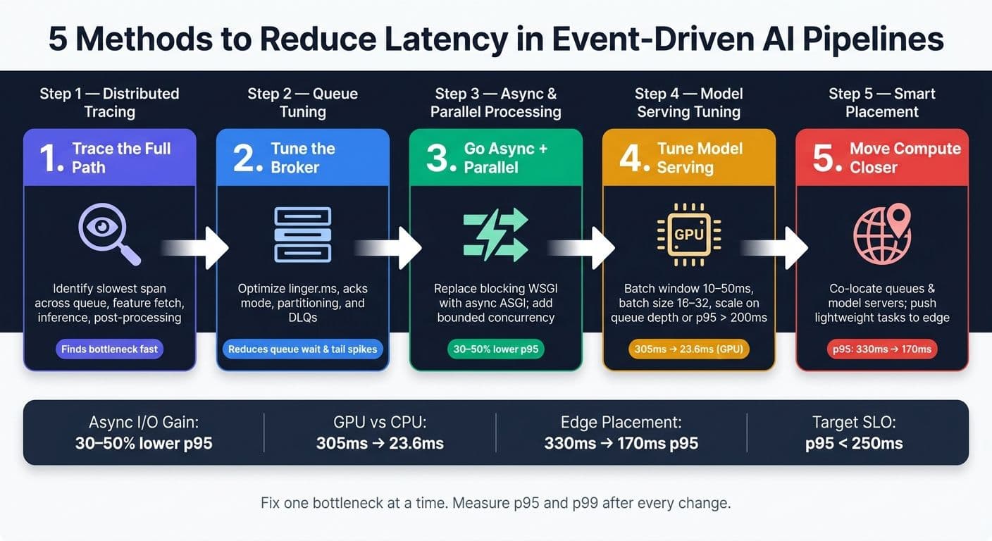
5 Methods to Reduce Latency in Event-Driven AI Pipelines
How to Reduce Latency in AI Applications (Real-World Techniques)
sbb-itb-903b5f2
Quick Comparison
| Method | Main problem it fixes | Typical gain |
|---|---|---|
| Distributed tracing | Hidden bottlenecks | Finds the slowest span fast |
| Queue tuning | Backlog and broker delay | Lower queue wait and tail spikes |
| Async + parallel work | Blocking I/O and idle time | 30%–50% lower p95 in some stacks |
| Model serving tuning | Slow inference and poor batching | Lower per-request model time |
| Smarter placement | Cross-region RTT and provider-side delay | Big drop in p95 when hops are cut |
If I were rolling this out, I’d make one change at a time, then recheck p95, p99, and cost per 1,000 events before moving to the next layer.
What Latency Looks Like in Event-Driven AI Pipelines
End-to-end latency is the total time from the moment an event enters the system - like a user clicking a product page - to the moment the AI response comes back. Component latency is the time spent inside one part of that path, such as the message broker, a feature store lookup, the model inference call, or an outbound API hop.
Here’s the plain-English version: users feel end-to-end latency. Engineers improve it by finding the part that’s dragging everything down.
When you measure latency, averages don’t tell the full story. Percentiles do.
- p50 shows the median
- p95 shows typical tail behavior
- p99 shows the slowest requests
That’s what users notice when a system feels snappy one moment and sluggish the next.
It also helps to track consumer lag, cold starts, and cross-region RTT. Lag means the queue is piling up. Cold starts can add 100 ms to more than 1 second. And network round-trip time (RTT) can stack up fast. Every call to an external feature store, risk API, or model server in another region adds more network time to the total.
In U.S.-focused systems, users often expect interactive AI features to respond in under 500 ms. That means even one cross-region hop can take a big bite out of the latency budget before inference even begins. Once that happens, tail latency can drift past target limits.
There’s also a clear tradeoff between throughput and responsiveness. Bigger inference batches help GPU use and increase total throughput, but they also make each event sit and wait longer. Databricks reported that on a single NVIDIA A100 GPU, pushing batch size to 64 increased throughput by 14x, while latency went up 4x.
Once you can see exactly where the delay shows up, tracing each hop is usually the first fix.
1. Track Event Flow With Distributed Tracing and Observability
Distributed tracing shows exactly where latency builds up across an event-driven pipeline: queue, feature fetch, inference, or delivery. Each event gets its own trace ID, and every step it passes through creates a timed span. Put those spans together and you get a clear record of where the time went. Instead of staring at a vague slowdown, you can point to the stage that's causing it and fix that part first.
Each span isolates a single hop, which makes the slow step stand out fast. You can see whether the delay comes from queueing, preprocessing, inference, or response delivery.
A practical way to use this data is to compare trace percentiles across queue wait, feature fetch, inference, and post-processing. Check p99 for the last 24 hours, line it up against your baseline, and then pull sample traces for the worst outliers. From there, look for the span that’s dragging the tail.
Tracing works even better when you pair it with queue-depth and consumer-lag metrics. That combo helps you spot the first saturated component instead of chasing symptoms downstream. Then you can sample only slow or failing traces, which keeps the signal clean.
Use the table below to map each span to the right optimization.
| Span Type | What It Measures | Optimization Target |
|---|---|---|
| Queue wait | Time sitting in Kafka, SQS, or Redis Streams | Consumer scaling, partition count |
| Feature fetch | Time querying feature stores or external APIs | Caching, co-location |
| Model inference | Time spent running the AI model | Batch size, hardware, model distillation |
| Post-processing | Time formatting or routing the response | Code optimization, async dispatch |
Use OpenTelemetry for instrumentation, then tag spans with queue_topic, model_name, tenant_id, and region. Those tags make it easy to isolate regressions by event type, tenant, or region when a p99 issue shows up.
2. Optimize Message Queues and Event Routing for Speed
Once you know where latency shows up in your pipeline, the next place to look is the queue. This is where a lot of teams win or lose speed. Batch size, persistence, and acknowledgment mode all shape how fast events move from producer to consumer.
Batch size and linger time are the first settings to check. They have a direct effect on delivery delay. If you're handling real-time inference, keep linger.ms close to zero. Larger batches make sense only when a bit of delay is fine.
Acknowledgment mode also has a big effect on latency. Stronger acknowledgments improve durability, but they also slow things down and can cut throughput. For lower-risk events like clickstream triggers, acks=1 gives you at-least-once delivery with less delay. Save acks=all for cases like financial transaction scoring or safety alerts, where durability matters more than raw speed.
Then there's routing design. Queue settings matter, but routing can make or break performance just as fast. Key-based partitioning keeps events in order, which sounds great on paper, but it can create hot partitions. If ordering doesn't matter, random or round-robin routing usually spreads load more evenly. And if bad events keep clogging the path, a dead-letter queue (DLQ) helps by pulling failed or malformed messages out of the main flow.
There's one more tradeoff worth calling out. Some latency-tuned setups increase the number of queue calls per event. When that happens, batch at the application layer if you can. It keeps queue calls down without slowing user-facing response time.
Use the table below to match queue settings to your latency goal.
| Configuration Lever | Low-Latency Setting | High-Durability Setting | Best For |
|---|---|---|---|
linger.ms (Kafka) | Very low | Higher | Real-time inference vs. batch analytics |
acks mode | acks=1 | acks=all | Low-risk events vs. critical events |
| Persistence | Async / in-memory | Sync, replicated | Ephemeral triggers vs. audit logs |
| Partitioning strategy | Random / round-robin | Key-based | Even load vs. strict ordering |
| Hot partition risk | Higher | Lower | Ordering vs. even load |
Once the queue is lean, the next bottleneck is how fast the system can process events while they're still in motion.
3. Use Async I/O, Streaming, and Parallel Event Processing
After you tune the queue, the next slowdown usually comes from work that sits around waiting while events are still in flight. Async I/O fixes that by keeping threads open for other requests. Instead of tying up one thread per request, an event loop can manage many in-flight requests with far fewer threads. Once queue wait drops, blocking I/O is often the next thing slowing you down. In practice, moving from a blocking WSGI stack to an async ASGI stack can cut p95 latency by 30–50% at the same throughput.
Streaming responses help on the user side and inside the system. Clients can start rendering tokens in 100–300 ms instead of waiting for the full output. That feels much faster, even when total generation time stays the same. Streaming over SSE, WebSockets, or gRPC also helps in multi-stage pipelines like pre-processing, inference, and post-processing. As soon as the first chunks show up, downstream consumers can begin their part of the job. That overlap between compute and I/O helps trim pipeline-wide p95.
Then there’s parallel event processing. This is what stops queueing time from taking over your tail latency when traffic jumps. More concurrent workers clear the queue faster. During a burst, doubling consumer instances can turn a 2–3 second queueing delay into under 200 ms, while inference time stays about 300–500 ms per event.
The catch is simple: more concurrency isn’t always better. If you add concurrency without backpressure, things can go sideways fast. Unbounded concurrency and missing circuit breakers can drain resources and push p99 into the 10–30 second range during surges. That’s why async I/O should go hand in hand with bounded concurrency, backpressure, and circuit breakers. The goal isn’t just lower latency on a calm day. It’s keeping p99 in check when traffic spikes and the system is under stress.
Once concurrency is under control, the next gains come from model serving, batching, and hardware.
4. Tune Model Serving, Batching, and Hardware Use
Once async I/O and concurrency are in good shape, the next place to look is how your model serves requests. In event-driven AI, total latency usually breaks into queueing time and inference time. So the job is simple in theory: keep the backlog under control, and keep each inference pass tight. In practice, even small setup mistakes can show up fast in p95 and p99, especially when traffic spikes.
Dynamic batching can improve GPU use and throughput without blowing past latency targets. When you group requests into a single inference pass, you lower the per-event cost of each forward call inside the pipeline. For real-time workloads, a good starting point is a 10–50 ms batch window and a max batch size of 16–32. That helps shrink the inference slice once queueing and async work are already under control.
Hardware choice also has a huge effect on tail latency. Moving from CPU to GPU can slash per-request latency. In one TorchServe tuning case, switching from CPU to GPU cut per-request latency from 305 ms to 23.6 ms, and FP16 cut p99 latency by 32% while increasing throughput by about the same amount.
Autoscaling needs the right trigger. If you scale only on CPU or GPU use, you often react too late - after the queue has already started to build. A better approach is to scale on:
- Queue depth
- Sustained p95 latency above 200 ms
These are common serving settings in Triton, TorchServe, and Ray Serve. Teams that skip them often leave latency gains and cost savings on the table. Once server-side tuning stops being the main bottleneck, the next lever is network placement.
If p99 still misses target after serving changes, the delay is usually coming from network hops.
5. Cut Network Latency With Smart Placement and Local Processing
Once serving is in good shape, the next bottleneck is often the network itself. At that point, the biggest gains usually come from where requests run: geography, edge routing, and local processing.
A simple rule helps here: put compute closer to where events start. If your queues and model servers run in the same region, round-trip time usually drops. Send traffic across regions, and delay stacks up fast. Edge locations in the same metro area can often stay in the 20–80 ms range, while cross-region or cross-continent centralized data centers can go past 150–250+ ms round trip. In one case, moving inference and queues into a closer region, then adding edge filtering, cut total p95 from about 330 ms to 170 ms even though inference time itself changed very little.
Sometimes even regional placement isn't close enough. That's when it makes sense to move simple work right to the edge, or even onto the device. Tasks like input validation, language detection, feature extraction, and basic anomaly detection are a good fit because they don't need a big central cluster to do useful work. More importantly, they remove extra hops from the event path. Local inference benchmarks show time-to-first-token usually landing between 50–200 ms, compared with 200–800 ms for cloud APIs under load. A big reason is that cloud APIs add provider-side queuing on top of normal network RTT.
The same logic matters during bursts. If all traffic flows into one central cluster, queues can pile up in a hurry and p99 can blow past SLOs. Regional sharding helps by splitting queue and inference stacks across regions like us-east-1 and us-west-2, so each one handles its own spike. Then add edge throttling - for example, rate limits or token buckets at the API gateway - to stop floods before they even hit the main cluster.
| Placement Strategy | Typical Round-Trip Latency |
|---|---|
| Client-side or on-device | <10–30 ms added |
| Edge locations in the same metro area | 20–80 ms |
| Regional data center | 60–120 ms |
| Cross-region centralized | 150–250+ ms |
Use central clusters for heavy inference. Push lightweight work to the edge or the device when you can.
Comparison Tables
These tables help you pick the lowest-latency fix that still matches your cost, durability, and ops budget. First, find the bottleneck. Then compare the tradeoffs that usually matter most: latency, cost, and setup effort.
| Tracing Setup | Overhead per Event | Cost per 1,000,000 Requests (USD) | Setup Complexity |
|---|---|---|---|
| Log-based correlation only | ~0–50 µs | $1–$10 | Low |
| Self-hosted (OpenTelemetry + Jaeger/Tempo) | ~50–500 µs (1–5% sampling) | $3–$20 | Medium |
| Managed platform (Datadog, New Relic, AWS X-Ray) | ~100–800 µs | $10–$100+ | Low–Medium |
Once visibility is in place, queue design is often the next fastest lever to pull.
| Queue / Broker | Typical p99 Latency | Throughput | Approx. cost per 1,000,000 messages (USD) |
|---|---|---|---|
| Apache Kafka / AWS MSK | 5–15 ms | ~1M+ msgs/sec per broker | $1–$15 |
| Amazon SQS (standard) | 100–500 ms | Elastic, managed | $0.40–$5.00 |
| Redis Streams / NATS | 100–500 µs to <5 ms | Very high (co-located) | $2–$25 |
Kafka gives you lower latency than managed serverless messaging, but it also asks for more day-to-day ops work.
If the server side is already tuned, network placement is usually the next thing that sets the limit.
| Pattern / Serving Mode | Typical Latency | vs. synchronous baseline | Incremental cost |
|---|---|---|---|
| Sync blocking I/O | ~300 ms (3 sequential calls) | Baseline | - |
| Async I/O per request | 120–180 ms | ~40–60% faster | Minimal |
| Streaming responses (SSE, WebSockets, gRPC streaming) | 50–200 ms time-to-first-token | Dramatically lower perceived latency | Negligible |
| Parallel fan-out | 250–350 ms (vs. ~800 ms sequential) | ~55–70% faster | Moderate (extra workers) |
| CPU-only serving (small models) | 50–300 ms | - | $2–$15 per 1M requests |
| GPU micro-batching (LLMs, batch size 4–32) | 20–200 ms | - | $5–$30 per 1M requests |
| Autoscaled / serverless (scale-to-zero) | 150–800 ms (cold start included) | - | $1–$10 per 1M requests |
| Placement Strategy | Typical Round-Trip Latency |
|---|---|
| Client-side or on-device | <10–30 ms added |
| Edge locations in the same metro area | 20–80 ms |
| Regional data center | 60–120 ms |
| Cross-region centralized | 150–250+ ms |
Where NanoGPT Fits in Event-Driven AI Workflows

After queue, serving, and network tuning are dialed in, the model-call layer is usually the last big integration point. If the rest of the pipeline is already running well, NanoGPT can sit between the event queue and inference as that model-call layer.
A worker can consume events like "new support ticket created" or "document uploaded" and then call NanoGPT for summarization, classification, image generation, or metadata extraction. That setup keeps AI latency away from the user-facing path. NanoGPT also supports background: true for long-running jobs and stream: true for SSE, so you can match the response pattern to the event type.
Once the worker path is set up, instrumentation should move to the top of the list. NanoGPT lets you attach up to 16 metadata pairs per request. Pass trace IDs and correlation IDs through those fields, then track queue wait time, model time, and retries as separate measurements. You can also use :fast, :speed, or :latency model suffixes to steer requests toward lower-latency options.
NanoGPT uses pay-as-you-go pricing, which works well for bursty event-driven pipelines. It stores data locally on the user's device, which matters when events include sensitive content like customer messages or internal documents. If you need stored responses, use store: true with x-encryption-key and retention_days: 0 to keep retention short.
Start with one event type, measure latency and reliability, and then expand from there once the path is steady.
How to Roll Out These Methods and Key Tradeoffs
Roll these methods out one bottleneck at a time. Start with distributed tracing and observability. Instrument every service, queue, and model call before you change anything else. Measure the slowest stage first. Once you know where the slowdown lives, move to queue tuning.
After you’ve pinned down the bottleneck, make changes in the order of lowest operational risk. In practice, that means: fix the queue first, then add async I/O and parallelism, then tune serving and batching, and only then look at placement changes.
That order matters. Queue tuning is usually low-risk and can deliver quick wins. Async changes and model serving add more overhead, so they make more sense after you’ve cleaned up upstream waste.
Use this table to pick the tradeoff that fits your system:
| Tradeoff | Lower Latency Option | Higher Throughput / Efficiency Option |
|---|---|---|
| Queue durability | In-memory queues - fast, weaker durability | Persistent queues - higher durability, higher latency |
| Batch size | Small batches (1–4) - low wait time | Large batches - higher p99 latency |
| Concurrency | Bounded worker pools - predictable, avoids saturation | High concurrency - more throughput, raises tail latency |
| Edge placement | Regional cloud endpoints - simpler to manage | True edge nodes - lowest latency, hardest to operate |
A simple rule of thumb:
- Use persistent queues for regulated events
- Use in-memory queues for low-risk paths under 100 ms
- Use multi-region deployment before moving to true edge nodes
Apply one change at a time, then remeasure p95 and p99 before you touch the next layer.
Conclusion
Reducing latency in event-driven AI is a systems problem across five layers: visibility, queue behavior, concurrency, inference serving, and network placement.
Here’s the catch: when you fix one layer, the next bottleneck tends to show up. Speed up the model, and queue delay starts to stand out. Clean up the queue, and network hops become the next drag. That’s why you need to keep measuring p95 and p99 after every change, not just once at the start.
Set a clear p95 end-to-end SLO like 250 ms, and instrument each stage so you can see exactly where the time is going.
Latency wins only count if the math still makes sense. Track cost per 1,000 events alongside p95.
Start with tracing, fix the biggest bottleneck, and then measure again before you move to the next issue.
FAQs
Which latency metric should I optimize first?
Start with a baseline for P50, P95, and TTFT. In many cases, TTFT matters most at the start because it shows how fast the AI begins to respond. And that has a big effect on how responsive the system feels to the user.
From there, tune based on your goal. Use TPOT for long-form output, or look at total response time to make sure the full reply hits your performance target.
How do I find the real bottleneck in my pipeline?
Start with a performance baseline. Track P50, P95, and TTFT, then run load tests with at least 1,000 requests to see when delays start to show up.
From there, check the usual suspects: model inference time, network delay, and synchronous API overhead. If you're working with streaming pipelines, look at consumer lag, checkpoint health, and state size. It also helps to use EXPLAIN to spot high-cardinality joins or wasteful data shuffles.
When should I move inference closer to users?
Move inference closer to users when your application needs real-time responsiveness. That matters for things like voice assistants, autonomous vehicles, and interactive customer service bots.
If network latency makes up a big share of end-user inference time, regional data centers or edge locations can reduce round-trip delays and improve responsiveness. This is especially useful when you're targeting response times below 100 milliseconds.