Scaling Depth vs. Width: Cost Trade-Offs
When building AI models, a key decision is choosing between scaling depth (adding layers) or scaling width (increasing layer size). Each option impacts performance, cost, and hardware demands differently:
-
Depth (more layers):
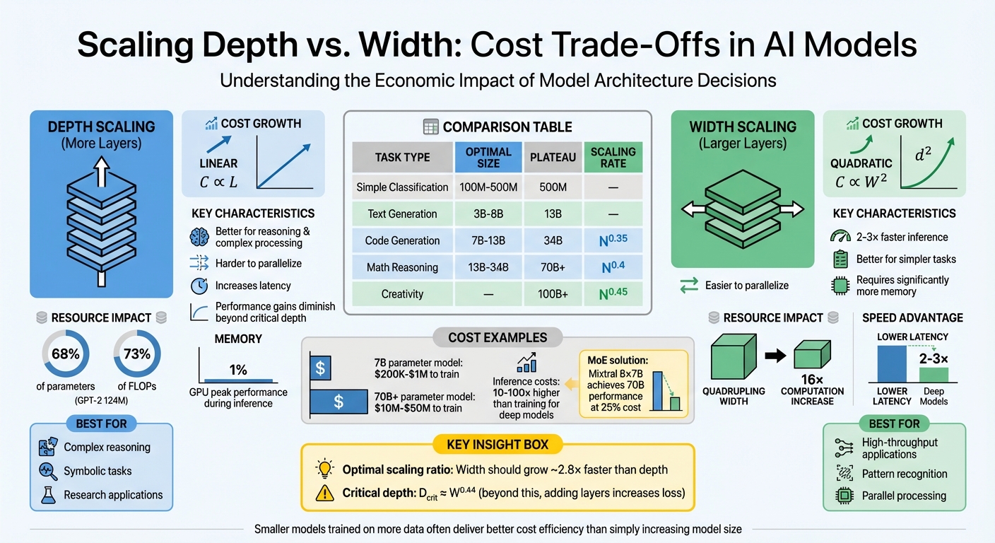
- Costs grow linearly.
- Better for tasks requiring reasoning or complex processing.
- Harder to parallelize, increasing latency.
- Performance gains diminish beyond a critical depth.
-
Width (larger layers):
- Costs grow quadratically.
- Easier to parallelize; faster inference and training.
- Better for simpler tasks or high-throughput applications.
- Requires significantly more memory.
Key insights:
- Deeper models excel at reasoning but are slower and less efficient for large-scale applications.
- Wider models handle parallel tasks better but are costlier due to memory and computation demands.
- Optimal scaling depends on the task, budget, and hardware.
For example, a 7B-parameter model can cost $200K–$1M to train, while scaling to 70B+ parameters could range from $10M–$50M. Techniques like Mixture of Experts (MoE) help reduce costs by activating only parts of a large model during inference.
Balancing depth and width is essential for achieving performance without overspending. Smaller models trained on more data often deliver better cost efficiency than simply increasing model size.
AI Model Scaling: Depth vs Width Cost and Performance Comparison
11 Scaling laws: basics (The Economics of Transformative AI, August 2025)
1. Scaling Model Depth
Adding more layers to a model doesn’t automatically translate to better performance. Research shows that increasing depth doesn’t create neatly layered representations, where early layers focus on syntax and deeper layers handle complex reasoning. Instead, most transformer layers make similar, incremental improvements through a process called "ensemble averaging".
Performance Impact
Initially, deep models were believed to divide tasks like syntax and semantics across layers. However, a January 2026 study of the Pythia-410m model using the FineWeb dataset found that 99.6% of tokens were updated evenly across its middle layers. This suggests that layers make small, similar adjustments rather than building distinct hierarchical representations.
Researchers also identified a critical depth ($D_{crit} \approx W^{0.44}$), beyond which adding layers actually increases loss, despite the additional parameters:
"Beyond $D_{crit} \sim W^{0.44}$ (sublinear in W), adding layers increases loss despite adding parameters - the Depth Delusion." - Md Muhtasim Munif Fahim and Md Rezaul Karim
For example, a study comparing 30 transformer architectures at the 7B parameter scale found that a 32-layer model outperformed a 64-layer model by 0.12 nats. Additionally, for tasks requiring context understanding, adding layers beyond 80–100 offers little improvement. The optimal scaling ratio suggests that width should grow roughly 2.8× faster than depth for the best results.
These performance challenges also affect the resources required to train and use deeper models.
Resource Usage
Adding layers increases computational costs linearly, following the formula $24nd^2 + 4n^2d$ per layer. In the GPT-2 (124M) architecture, transformer blocks - which define the model’s depth - account for 68% of the total parameters and 73% of the total FLOPs. Training costs are further amplified because the backward pass requires twice as much computation as the forward pass.
Memory usage becomes a critical bottleneck as depth increases. During inference, where tokens are generated one at a time, the model must load the weights for every layer from memory. This memory-bound process operates at just 1% of a GPU’s theoretical peak performance. For instance, training a 124M parameter model on 300 billion tokens using an 8× A100 node at 30% Model Flops Utilization takes approximately 3.46 to 4 days.
Cost Efficiency
The high memory and computational demands of deeper models directly affect cost efficiency. Scaling depth is less cost-effective than scaling width. Computational costs adhere to the 6ND approximation (6 × Parameters × Tokens), meaning each additional layer adds a fixed FLOP cost. For applications with heavy inference demands - such as 1 billion requests - it may be more economical to train smaller, shallower models on larger datasets rather than simply increasing depth.
The industry is moving away from extreme depth. For instance, GPT-4 reportedly relies on wider hidden layers instead of significantly increasing depth to avoid training inefficiencies. Additionally, inference costs for deeper models can be 10× to 100× higher than smaller models, as each added layer increases memory traffic during decoding.
Balancing depth, width, and computational efficiency is key to designing cost-effective and high-performing model architectures.
2. Scaling Model Width
Increasing a model's width means expanding its hidden dimension, which enhances its ability to represent complex ideas through high-dimensional spaces. This ensures that token representations remain distinct and less likely to overlap. For example, GPT-3 operates with a width of 12,288 dimensions, LLaMA-3.2 405B reaches 16,384, and DeepSeek R1 uses around 7,168 dimensions. Shifting focus from depth to width impacts both performance and resource demands in unique ways.
Performance Impact
Width plays a critical role in how effectively a model learns and processes information. Wider architectures spread learning across fewer layers, which reduces redundancy often seen in deeper models. In deep setups, later layers sometimes end up merely copying earlier ones, which wastes capacity. A wider design, on the other hand, allows for better role assignment - like keeping the subject and verb distinct - making it ideal for handling multi-step reasoning.
Another advantage is speed. Unlike deeper models, which require longer sequential paths and slow down training, wider models allow for more efficient parallel processing. This helps avoid gradient bottlenecks, which can hinder learning. As Noel Benji explains:
"For large-scale LLMs, widening hidden layers is often a more effective scaling strategy than adding excessive depth".
Resource Usage
Expanding width comes with a steep price: computational and memory costs increase quadratically ($d^2$). For instance, quadrupling a model's width leads to a 16× increase in computation requirements. In standard transformer designs like GPT-2 (124M), the MLP blocks already take up about twice the parameters of attention blocks. This quadratic growth in costs makes width a more resource-intensive choice compared to simply adding depth, which scales linearly.
Cost Efficiency
The high computational and memory demands of wider models also bring unique cost challenges. During the memory-intensive decoding phase, width's quadratic scaling becomes especially expensive. However, techniques like Mixture of Experts (MoE) architectures can help reduce these costs. For example, Mixtral 8×7B achieves the performance of a dense 70B model at just 25% of the cost.
For those working within fixed compute budgets, the Chinchilla scaling law suggests an optimal 20:1 token-to-parameter ratio. Yet, newer models like LLaMA-3 have pushed this to a 200:1 ratio, showing that smaller, narrower models trained for longer periods can sometimes outperform larger ones in terms of cost efficiency.
How Each Approach Affects Performance
After examining resource usage and cost efficiency, it’s time to see how scaling model depth and width impacts performance. The relationship here isn’t straightforward - performance gains depend heavily on the type of task.
Reasoning and creative tasks benefit the most from larger models. For creativity-related tasks, performance scales at a rate of _N_⁰·⁴⁵, with improvements continuing even beyond 100 billion parameters. Mathematical reasoning follows closely, scaling at _N_⁰·⁴, but it starts to plateau after hitting 70 billion parameters. On the other hand, basic language understanding caps out much earlier, around 13 billion parameters, with a slower scaling rate of _N_⁰·²⁵. For simpler tasks like classification, diminishing returns set in as early as 500 million parameters.
Here’s a quick breakdown of scaling rates and performance plateaus for different tasks:
| Task Type | Optimal Model Size | Performance Plateau | Scaling Rate |
|---|---|---|---|
| Simple Classification | 100M – 500M | 500M parameters | - |
| Text Generation & Chat | 3B – 8B | 13B parameters | - |
| Code Generation | 7B – 13B | 34B parameters | _N_⁰·³⁵ |
| Mathematical Reasoning | 13B – 34B | 70B+ parameters | _N_⁰·⁴ |
| Knowledge Tasks (MMLU) | - | 30B+ parameters | _N_⁰·³ |
| Creativity | - | 100B+ parameters | _N_⁰·⁴⁵ |
Wider models have an edge when it comes to speed. They take better advantage of hardware parallelization, running 2–3 times faster than deeper models with similar accuracy levels. However, as noted in Section 1, simply stacking more layers - what’s often called the "Depth Delusion" - can actually hurt performance once you pass a certain threshold. More layers don’t always mean better results.
For specialized tasks, smaller models can sometimes match or even outperform larger ones with targeted fine-tuning. In areas like medical diagnostics, where data is limited, scaling up can lead to overfitting. In these cases, simpler models can hold their own while using far fewer resources. Microsoft CEO Satya Nadella put it this way:
"Progress in generative AI should be measured in 'token per dollar per watt', as opposed to metrics focusing only on accuracy- or cost".
These trends highlight the importance of tailoring model architecture to the specific needs of an application, balancing computational demands with performance goals.
sbb-itb-903b5f2
Resource Requirements and Cost Comparison
The hardware needed for scaling depth versus width varies significantly. When scaling depth (adding more layers), parameters and memory requirements grow linearly. However, scaling width (increasing embedding dimensions) leads to a quadratic rise in parameters. This is especially pronounced in attention and MLP layers, where doubling the width results in a fourfold increase in memory usage.
As models grow, the memory bottlenecks shift. Smaller models primarily consume GPU memory for activations during forward and backward passes. In contrast, larger models face constraints from parameters and optimizer buffers. For example, the AdamW optimizer stores not only the model parameters but also two additional buffers for moment estimates, requiring approximately params × 4 bytes (fp32) × 3. These memory demands directly influence both training and operational costs.
Training compute costs can be estimated using the 6ND approximation, where N is the number of parameters and D is the number of training tokens. Forward passes require about 2ND FLOPs, while backward passes need 4ND FLOPs. For large models, memory bandwidth becomes a critical factor - parameters must be loaded quickly enough to avoid bottlenecks, which can significantly impact operational expenses beyond peak performance.
The financial implications of these compute demands are substantial. Local infrastructure costs can be steep compared to cloud-based solutions. For example, by 2026, deploying competitive local models will require $80,000 to $100,000 in specialized GPU hardware. However, optimization can drastically reduce these costs. Meituan, a Chinese food delivery platform, successfully optimized a 7B parameter model to match the performance of a 72B model for restaurant recommendations. This reduced VRAM requirements from 140 GB to just 14 GB, enabling deployment on a single RTX 4090 GPU (around $1,800) instead of a multi-GPU cluster costing over $60,000. This approach cut infrastructure costs by roughly 90%.
Cloud-based solutions offer another cost-saving alternative. Pay-as-you-go API access avoids the need for upfront hardware investments. For instance, NanoGPT provides granular pricing at $0.05 per 1M input tokens and $0.40 per 1M output tokens, compared to GPT-4.1’s $2.00 and $8.00 respectively. Additionally, prompt caching can reduce costs by up to 90%, making it an attractive option for projects with variable usage patterns .
Scaling for Large Applications
As applications grow to handle billions of requests daily, deploying AI models at such scale requires careful planning. One key decision revolves around balancing depth and width in your infrastructure. Scaling for width allows for better parallelization across hardware, distributing workloads across multiple GPUs. On the other hand, increasing depth means adding more sequential computational steps, which can significantly increase inference latency. For applications where quick response times are non-negotiable, this sequential delay becomes a critical issue.
When working with trillion-parameter models, research has identified a tipping point: once depth surpasses the logarithm of width ($L > \log_3 d_x$), the trade-offs between these two dimensions become almost equal in performance. This finding suggests that for trillion-scale models, expanding width is generally more effective than simply stacking additional layers. As Levine et al. emphasized:
"At trillion-scale parameter counts, optimal architectures should grow width rather than depth".
But scaling width comes with its own challenges. Wider models activate every parameter per token, requiring around 2N FLOPs per token. This makes the cost of serving wider models increase linearly, with memory bandwidth quickly emerging as a major bottleneck. For high-volume applications processing millions of requests daily, these per-token costs can accumulate quickly, forcing teams to carefully weigh performance against expense.
One way to manage costs is through overtraining smaller models. For instance, in 2024, Meta unveiled Llama-3-70B, trained on 15 trillion tokens - a token-to-parameter ratio of 200:1, far surpassing the standard 20:1 Chinchilla-optimal ratio. Similarly, Mistral AI trained its 7B-parameter model on about 8 trillion tokens, achieving a 57× overtraining ratio. Both companies made significant upfront investments in training to reduce inference costs, which can be up to 100× higher than training costs in high-demand scenarios.
An emerging architecture that addresses these challenges is the Mixture of Experts (MoE). This design increases effective width by activating only a subset of parameters for each token. MoE offers a practical compromise, combining the expressive power of large models with the efficiency needed for large-scale deployments.
Advantages and Disadvantages
Here's a breakdown of the trade-offs between depth and width scaling in AI models:
Depth scaling offers exponential improvements in expressivity but comes at the cost of increased sequential latency. Deep, narrow models can mimic the performance of wide, shallow ones with only a polynomial overhead. This makes depth scaling a great choice for tasks involving complex reasoning or symbolic computation. However, deeper models are harder to parallelize across hardware, and excessive depth can significantly lower Model Flop Utilization (MFU).
Width scaling, on the other hand, provides polynomial improvements in representational capacity and excels in parallelization. Wider models distribute workloads more effectively across GPUs, reducing inference latency by 2–3× compared to deep, narrow models with similar accuracy. This makes width scaling ideal for high-throughput applications and simpler pattern recognition tasks. The trade-off? Wider models require activating all parameters for each token, which leads to linearly increasing inference costs.
| Factor | Depth Scaling | Width Scaling |
|---|---|---|
| Performance Gain | Exponential expressivity gains | Polynomial gains in representational capacity |
| Flexibility | High; can approximate wide models with polynomial overhead | Lower; requires exponential width to approximate deep models |
| Hardware Efficiency | Harder to parallelize; increases sequential latency | Easier to parallelize; better for high-throughput hardware |
| Resource Demands | Increases initialization time; may reduce MFU if excessive | Increases memory footprint for activations and parameters |
| Best For | Reasoning, symbolic tasks, and high-complexity functions | Simple classification, pattern recognition, and parallel processing |
These comparisons illustrate the challenges and decisions that come with scaling AI models. As noted by Emergent Mind:
"Deep architectures with modest width are often exponentially more powerful than shallow, ultra-wide ones for a broad class of tasks".
However, as models grow to trillions of parameters, width scaling becomes the more practical approach. Cost considerations often guide these architectural decisions, pushing teams to weigh depth and width carefully based on their goals and available resources.
Conclusion
Depth and width scaling bring unique cost-performance trade-offs, making it essential to align architectural choices with specific application needs and budget limits.
Deep, narrow models shine in tasks requiring complex reasoning and research, thanks to their exponential expressivity. Meanwhile, wide, shallow models are better suited for parallelized, high-throughput tasks, often delivering 2–3× lower inference latency. Striking the right balance between depth and width is key to optimizing both performance and cost efficiency.
Budget constraints play a crucial role in these decisions. As model size grows, so do training and inference costs. Smaller models in the 7B parameter range can deliver roughly 79% of peak performance at a fraction of the cost of larger models. For simpler tasks like basic classification or edge deployments, 1B–3B models can provide faster returns on investment. On the other hand, applications requiring sub-300 ms response times should focus on models under 10B parameters to minimize sequential latency. Techniques like prompt caching can further enhance cost efficiency.
As Local AI Master aptly stated, "For fixed compute budgets, smaller models trained on more data often outperform larger models trained on less data". This insight applies whether scaling is achieved through depth or width. Additionally, Mixture of Experts (MoE) architectures are making strides in efficiency by enabling trillion-parameter models to operate at the computational cost of 100B dense models, thanks to selective "expert" activation per token.
NanoGPT simplifies experimentation and deployment with its pay-as-you-go approach, removing upfront subscription costs. This flexibility allows teams to test various model sizes - from compact options like the 3.8B Phi-3 Mini to cutting-edge models - without long-term commitments. Choosing the right model depends on factors like task complexity, latency requirements, and cost-per-token considerations.
FAQs
How do I decide whether to scale depth or width for my use case?
When deciding whether to scale a model in depth or width, it’s essential to consider your specific goals, resources, and use case. Deeper models excel at learning complex, hierarchical patterns, but they typically demand more computational power. On the other hand, wider models can boost performance with fewer layers, though they might consume more memory.
Often, striking a balance between depth and width yields the best results. Deeper models are well-suited for tackling intricate tasks, while wider models are a better fit for simpler problems. Carefully weigh the trade-offs in performance, cost, and latency to determine the most effective strategy for your needs.
What is 'critical depth,' and how can I tell when adding layers will hurt performance?
'Critical depth' refers to the point in a neural network where adding more layers no longer improves performance - in fact, it can start to make things worse. When a network reaches this stage, the extra layers become redundant, which limits the model's ability to learn effectively.
How can you spot this? Keep an eye on the loss. If adding layers no longer reduces the loss - or worse, causes it to rise - it’s a clear sign that the network is experiencing diminishing or even negative returns from the additional complexity.
How can I cut inference cost at scale without losing too much quality?
To manage inference costs effectively at scale while keeping quality intact, it's crucial to match the model's complexity to the specific task. Using smaller, task-focused models can slash costs by as much as 90% without significantly affecting performance. Other cost-saving strategies include optimizing prompts, caching commonly used outputs, and leveraging compute-efficient models to strike a balance between cost and quality. On top of that, applying rate limits and throttling can help manage expenses during periods of high traffic.