Sparse Data in Scientific Simulations

Most large simulation matrices are almost all zeros, so storing them as dense arrays wastes huge amounts of memory and time. I’d sum it up like this: use sparse storage when each row touches only a small set of neighbors, match the format to the solver, and check whether the cost of extra indexing is worth it for your workload.

Here’s the short version:

• I see sparse data as the reason many large PDE, FEM, CFD, and MPM runs fit on available hardware at all.
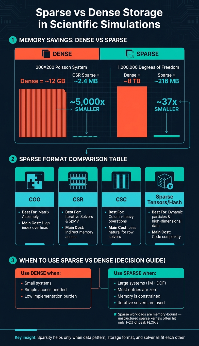
• Dense storage can explode fast: a 200 × 200 Poisson system can jump to about 12 GB dense, while CSR can cut that to about 2.4 MB.
• At 1,000,000 degrees of freedom, dense storage can reach about 8 TB, while sparse storage can stay near 216 MB.
• The main formats split by job:
  • COO for assembly
  • CSR for row-based solver work and SpMV
  • CSC for column-based work
  • Sparse tensors / hash-based layouts for higher-dimensional or dynamic state data
• Sparse methods save memory, but they also add index overhead, irregular memory access, and more code work.
• Solver speed often depends more on memory bandwidth than peak math rate, especially for SpMV in CG and other Krylov methods.
• A solid pipeline is usually simple in outline: inspect the pattern, pick the format, assemble in stages, and test against a small dense case.

If you work on simulation code, the main point is simple: sparsity helps only when the data pattern, storage format, and solver all fit each other. That’s the lens I’d use for the rest of the article.

Sparse matrices powering three pillars of science: simulation, data, and learning (part 1)

sbb-itb-903b5f2

Quick comparison

Item	Best fit	Main upside	Main cost
Dense arrays	Small systems	Simple access	Memory blows up fast
COO	Matrix assembly	Easy to add entries	High index overhead
CSR	Iterative solvers, SpMV	Low storage, row-wise speed	Indirect access
CSC	Column-heavy operations	Good for column traversal	Less natural for row solvers
Sparse grids	High-dimensional problems	Far fewer grid points than full tensor grids	Harder indexing
Hash-based sparse layouts	Dynamic particle/grid methods	Works well for active regions only	More code complexity

That’s the core story: sparse data is not just about saving space. It changes how you assemble, solve, benchmark, and document a simulation workflow.

Benefits and Tradeoffs of Sparse Representations

Memory Savings and Faster Solvers

In stencil and mesh-based solvers, each grid point or element usually interacts with only a small set of neighbors. That’s why sparse storage works so well: it keeps the physics you need and drops the wasted work tied to zero entries.

In practice, that can be the line between a model that fits in memory and one that won’t run at all. When memory is tight, sparse storage isn’t just nice to have. It decides whether the job can even start.

The same idea carries over to solver speed. Sparse matrix-vector multiplication skips zeros, so iterative solvers spend each step doing useful arithmetic instead of plowing through empty entries. And because iterative solvers call SpMV at every step, cutting work per iteration adds up fast.

Those gains matter even more once models outgrow a single node or GPU.

Scalability, Cache Behavior, and Energy Costs

Sparse layouts can help keep large adaptive simulations inside single-GPU memory limits. In distributed HPC settings, they can also cut the amount of data sent across MPI boundaries.

There’s a catch, though. Sparse codes are usually memory-bound, not compute-bound. They often run below peak FLOP/s because indirect indexing leads to irregular memory access and cache misses. Put simply, the processor has to do extra lookups before it can use each value, and that slows things down.

That same irregular access pattern is also why sparse software is tougher to build and tune. You save memory and cut some work, but you pay for it in data movement and code complexity.

When Sparse Data Adds Complexity

Sparse storage is not free. Every nonzero entry needs extra metadata, such as row indices, column indices, or offset pointers. A 64-bit index plus a 32-bit value can add a lot of overhead.

Here’s the tradeoff at a glance:

Feature	Dense	Sparse (e.g., CSR)
Memory	$O(N^2)$ - grows quadratically	$O(N + nnz)$ - scales with nonzeros
Access Pattern	Sequential, predictable	Indirect, irregular; prone to misses
Implementation Burden	Simple 2D arrays	Multiple arrays, graph builders, format conversions
Best Use Case	Small, dense systems	Large, sparse simulation systems

Building sparse structure also takes more work than filling a dense array. Many codes first build a dynamic graph or mask, then populate the matrix values later. So the payoff from sparse methods depends a lot on reuse. If you build the structure once and use it many times during the solve, the trade starts to make sense.

The next step is choosing a format that fits the solver and the sparsity pattern.

Core Sparse Formats Used in Simulation Codes

Storage format shapes assembly speed, solver efficiency, and hardware behavior.

CSR, CSC, and COO for Sparse Matrices

Each format works best at a different point in a simulation workflow.

COO (Coordinate) is the most direct format. It stores each nonzero as a (row, column, value) tuple, which makes it a good fit for assembly. If the same coordinate shows up more than once, those duplicates are summed during conversion.

That assembly-first path usually ends with a conversion to CSR or CSC for the solve step.

CSR (Compressed Sparse Row) stores row offsets in row_ptr, which cuts index storage by a lot. It's the standard choice for SpMV and iterative solvers.

CSC (Compressed Sparse Column) is the column-based version of CSR. It compresses column indices instead of row indices, so it tends to work better when operations slice columns or loop through them instead of rows.

In practice, many simulation codes follow a simple two-step pattern: build in COO, then convert to CSR before passing the matrix to the solver. Kratos Multiphysics uses a close variation of this idea. It starts with SparseGraph or SparseContiguousRowGraph to define the sparsity pattern from element connectivities, then builds a CsrMatrix for numerical assembly and SpMV work. That split keeps assembly flexible and makes the solve phase faster.

The same idea also carries over to higher-dimensional state data.

Sparse Tensors and High-Dimensional Layouts

Sparse tensors take these same storage ideas into higher-dimensional simulation data and coupled workloads, where only part of the state is active.

They can also help GPU kernels run faster when the nonzero pattern lines up with the hardware layout. Think of it like packing only the tools you’ll use instead of hauling the whole toolbox.

Use the table below to match each format to the job:

Format	Memory Overhead	Best Operations	Access Pattern	CPU/GPU Suitability
COO	High (2 indices per value)	Matrix assembly, incremental updates	Random / tuple-based	CPU assembly
CSR	Low (1 index + row offsets)	SpMV, row slicing, iterative solvers	Row-major	CPU & GPU (solvers)
CSC	Low (1 index + col offsets)	Column slicing, matrix-matrix products	Column-major	CPU & GPU (solvers)
Sparse Tensor	Variable (metadata-based)	Multiphysics, batching, coupled workloads	High-dimensional / block-contiguous	GPU batching

Once the format is fixed, the next step is picking algorithms that make the most of it.

Algorithms and Implementation Techniques

Once the storage format is set, the next step is simpler to ask than to answer: which algorithms should run on top of it? That choice has a big effect on runtime, memory use, and how well the code maps to CPU or GPU hardware.

Iterative Solvers for Large Sparse Systems

For large sparse systems from FEM or CFD workflows, Conjugate Gradient (CG) and other Krylov methods are usually the first place people start. And for good reason. These methods spend most of their time in sparse matrix-vector multiply, or SpMV, so runtime is usually limited by memory bandwidth, not raw FLOP/s. On modern hardware, unstructured sparse kernels often hit only 1–2% of peak FLOP/s.

That sounds low, but it’s normal. Sparse workloads don’t feed hardware the way dense linear algebra does.

Preconditioning is the part that turns iterative solvers from a nice idea into something you can use. Without it, convergence can be painfully slow, and in some cases it can stall out completely. One method getting more attention for GPUs is ParILU. It’s a parallel Incomplete LU factorization that swaps serial elimination for parallel fixed-point updates, which helps avoid the serial dependencies that make classic ILU tough to run well on GPUs.

If you don’t want to build this stack from scratch, you don’t have to. Ginkgo, hypre, and PETSc/Trilinos all offer production-ready solvers and preconditioners.

Sparse Grids and Adaptive Approximation

Sometimes the hard part isn’t matrix size. It’s dimensionality.

That’s where sparse grids come in. Instead of working like iterative solvers on linear systems, sparse grids target high-dimensional discretization. The idea is to avoid full tensor grids, which blow up fast as dimension count climbs, and replace them with structured subsets that keep most of the accuracy while using far less work.

In practice, sparse grids can reduce degrees of freedom a lot compared with full tensor grids, without much loss in accuracy.

The catch is the implementation. The indexing schemes are tricky, and the method tends to work best when the underlying function is smooth. So the payoff can be strong, but you have to earn it.

Steps for Building a Sparse Simulation Pipeline

After choosing the method, the next check is whether the sparse format matches the access pattern. That part gets overlooked all the time. A good sparse pipeline usually follows the same basic flow, no matter what physics you’re solving.

• Inspect the sparsity pattern first. Start with a spy plot. A banded matrix behaves nothing like a scattered one. This is also where you decide if reordering, such as Reverse Cuthill-McKee, is worth using to improve cache locality.
• Choose the format based on access pattern. Use CSR for row-wise solver work, COO as an intermediate assembly format, and hash-based indexing for GPU-heavy methods like the Material Point Method (MPM). It also helps to measure the dense-to-active ratio before committing to a sparse layout.
• Assemble in stages. Define the nonzero pattern with a graph object before filling in the numerical values. That makes assembly thread-safe.
• Benchmark against a dense reference. Test the sparse solver on a small problem where a dense solve is still practical. It’s one of the easiest ways to catch format bugs, convergence trouble, and precision loss before those issues spread through a full-scale run.

The table below gives a side-by-side view of the main method families across the factors that matter most in day-to-day work:

Method	Typical Use Case	Accuracy	Scalability	Hardware Fit	Implementation Difficulty
Iterative (CG/Krylov)	Large-scale FEM/CFD	High (tolerance-based)	Excellent	CPU & GPU	Moderate
Direct Solvers	Ill-conditioned systems	Very High	Limited	CPU (multi-core)	High
Algebraic Multigrid	Optimal $O(N)$ scaling	High	High	CPU & GPU	Very High
Sparse Grids	High-dimensional interpolation	Moderate–High	High	CPU	High
Matrix-Free	Exascale simulations	High	Maximum	GPU/Vector	High
Hash-based Indexing	Dynamic particles (MPM)	High (exact)	Very High	Excellent (GPU)	High

AI-Assisted Workflows and Key Takeaways

Using NanoGPT for Analysis and Documentation

Once the pipeline finishes, the job isn’t over. You still need to turn logs, solver output, and benchmark results into documentation that other people can follow and repeat.

Sparse simulations don’t just spit out particle or grid data. They also generate solver settings, logs, and performance metrics that need to be written down for reproducibility. NanoGPT can help summarize benchmark logs and explain why certain format choices were made. It keeps data local and uses pay-as-you-go pricing.

This is where AI tends to help most: analysis, documentation, and reporting.

Workflow Step	Action	Tools / Techniques
Simulation Output	Generate raw particle or grid data	MPM solvers, CFD frameworks
AI-Assisted Analysis	Compare runs, flag anomalies, and summarize solver behavior	NanoGPT
Documentation and Reporting	Summarize logs and draft final reports	NanoGPT

One thing matters a lot here: give the model exact benchmark numbers, format names, and solver settings. If your input is vague, the summary will be vague too.

Conclusion: Key Points About Sparse Data

Sparse data makes large simulations possible when most of the domain is inactive. There’s no single format that wins in every case. The best sparse pipeline depends on the physics, the hardware, and the solver, and those choices need to be documented clearly.

FAQs

When should I use sparse instead of dense storage?

Use sparse storage when your data set has lots of default values, usually zeros, that would just eat up memory for no good reason. It’s a smart fit for large scientific simulations because it stores only the non-zero entries and skips wasted work on zero values.

This approach works best when interactions stay local or when material properties appear only in certain parts of a grid. In those cases, sparse structures can cut memory use and improve processing time compared with dense storage.

How do I choose between COO, CSR, and CSC?

Choose the format based on what you need the matrix to do:

• COO if you're building the matrix or changing entries in place
• CSR for fast row slicing, arithmetic, or matrix-vector multiplication
• CSC when you do a lot of column slicing or other column-based work

A common pattern is simple: start in COO, then convert to CSR or CSC when you're ready to use it.

Why are sparse solvers often memory-bound?

Sparse solvers are often memory-bound because their arithmetic intensity is low. Put simply, they do only a small number of floating-point operations for each byte pulled from memory.

Sparse matrix-vector multiplication is one of the clearest examples. Its work-to-data-movement ratio is very low, so the solver keeps reloading nonzero values and their indices again and again. That means performance is usually capped by memory bandwidth, not by the raw processing speed of the CPU or GPU.