Vanishing Gradients in RNNs: Causes and Fixes
Vanishing gradients can cripple RNNs, making it nearly impossible for them to learn long-term patterns. This happens when gradients shrink exponentially during backpropagation, especially in long sequences or when using certain activation functions like sigmoid and tanh. The result? RNNs struggle to retain information from earlier timesteps.
Here’s what causes the problem and how to fix it:
-
Causes:
- Small derivatives from activation functions (e.g., sigmoid, tanh).
- Repeated multiplications in long sequences.
- Poor weight initialization.
-
Solutions:
- Use LSTMs or GRUs to maintain gradient flow.
- Replace sigmoid/tanh with ReLU or Leaky ReLU.
- Apply gradient clipping to stabilize training.
- Initialize weights properly with methods like Xavier or He.
For tasks requiring long-term memory, LSTMs are highly effective due to their gating mechanisms. For shorter sequences, switching activation functions or improving weight initialization can help. Gradient clipping is a quick fix for training instability but doesn’t fully solve vanishing gradients.
Main Causes of Vanishing Gradients in RNNs
Activation Functions (Sigmoid and Tanh)
The sigmoid and tanh activation functions are major contributors to the vanishing gradient problem. These functions compress their outputs - sigmoid to a range of 0 to 1, and tanh to -1 to 1. The issue lies in their derivatives. For sigmoid, the maximum derivative is only 0.25, while tanh's derivative peaks at 1.0, and only when the input equals zero. In most cases, these derivatives are smaller than 1.0, which causes gradients to shrink during backpropagation.
When using Backpropagation Through Time (BPTT), these small derivatives are multiplied repeatedly. Michael Brenndoerfer, author of the Language AI Handbook, explains:
The Jacobian factors into two components: The diagonal matrix... captures how the tanh activation attenuates the gradient. Since $\tanh'(z) \le 1$ everywhere, this matrix can only shrink gradients, never amplify them.
This problem worsens due to the saturation effect. When inputs to these functions are very large or very small, the outputs flatten, and the derivatives approach zero. This essentially stops the gradient flow for those neurons. Pranav Pillai, Co-Founder of Lex Analytics, highlights this:
Each partial derivative of hidden states is a function of the activation function used... the magnitude of each derivative of hidden states is less than 1, the result is that the entire gradient approaches 0 as the number of samples increase.
These limitations of sigmoid and tanh are further compounded by challenges with sequence length, which we'll discuss next.
Repeated Multiplications in Long Sequences
Long sequences present another challenge due to the chain rule product structure. Gradients for earlier timesteps require multiplying the Jacobian matrices from all subsequent steps. For instance, in a sequence of 1,000 tokens, the input at the first step undergoes over 1,000 matrix multiplications. Combined with small activation derivatives, this quickly diminishes gradients.
The rate of gradient decay depends heavily on the spectral radius, which is the largest eigenvalue of the weight matrix. If the spectral radius is less than 1, the gradient diminishes exponentially as the sequence length increases. When paired with activation derivatives typically below 0.6, this leads to rapid gradient decay over time.
The table below illustrates how decay factors impact gradient magnitudes over multiple steps:
| Decay Factor ($\gamma$) | Magnitude after 10 steps | Magnitude after 20 steps | Magnitude after 50 steps |
|---|---|---|---|
| 0.9 (Mild) | ~0.348 | ~0.121 | ~0.005 |
| 0.7 (Moderate) | ~0.028 | ~0.0008 | ~$1.7 \times 10^{-8}$ |
| 0.5 (Typical RNN) | ~0.0009 | ~$9.5 \times 10^{-7}$ | ~$8.8 \times 10^{-16}$ |
| 0.3 (Severe) | ~$5.9 \times 10^{-6}$ | ~$3.4 \times 10^{-11}$ | ~$7.1 \times 10^{-27}$ |
As the table shows, even mildly small decay factors can lead to gradients that are effectively zero after just a few steps.
Poor Weight Initialization
Another contributing factor is improper weight initialization. If weights are initialized too small, the repeated multiplications in RNNs cause gradients to shrink exponentially. This issue is particularly problematic because RNNs reuse the same weight matrix at every timestep.
Naive initialization methods, such as drawing weights from a Gaussian distribution $W \sim N(0,1)$, fail to consider the architecture of the network. This leads to a variance imbalance, where activations either explode or vanish as they propagate through layers, disrupting gradient flow.
Modern techniques like Xavier initialization (for tanh and sigmoid) and He initialization (for ReLU) address these issues by scaling weights based on the number of input and output neurons. The formulas are:
- Xavier: $Var(W) = \frac{2}{n_{in} + n_{out}}$
- He: $Var(W) = \frac{2}{n_{in}}$
These methods help maintain balanced variance, ensuring gradients don't vanish or explode. Without proper initialization, lower-layer parameters barely update, while upper layers continue to change, leading to a network that struggles to learn even basic features.
Solutions for Vanishing Gradients in RNNs
Gradient Clipping
Gradient clipping is a technique used during backpropagation to cap gradient values, preventing instability that can lead to exploding or vanishing gradients. This method helps avoid loss spikes and NaN values, which are common when gradients become unstable, especially in the early training stages.
The process involves setting a threshold for gradient magnitudes. For example, in language modeling, researchers have achieved top results with maximum gradient norms as low as 0.25. More commonly, practitioners use values like 1.0 or 5 for max_grad_norm. By doing so, gradient magnitudes are reduced from extreme ratios (e.g., over 10,000) to manageable levels, ensuring effective learning across all timesteps.
When clipping, opt for norm clipping over value clipping. Norm clipping scales the entire gradient vector proportionally, preserving its direction, which is essential for learning. In PyTorch, you can use torch.nn.utils.clip_grad_norm_(model.parameters(), max_norm), while TensorFlow provides tf.clip_by_global_norm(gradients, max_grad_norm) for the same purpose. It's also a good practice to monitor gradient norms layer by layer in real-time to catch instability before it causes the model to diverge.
Another approach to mitigate vanishing gradients involves choosing the right activation functions, which we’ll discuss next.
Using ReLU or Leaky ReLU Instead of Sigmoid/Tanh
ReLU activation functions are effective in addressing vanishing gradients due to their constant gradient property. For positive inputs, ReLU's derivative is always 1, which ensures steady gradient flow during backpropagation. As Juan C Olamendy, Senior AI Engineer, puts it:
ReLU helps mitigate the vanishing gradient problem because the gradient is either 0 (for negative inputs) or 1 (for positive inputs). This ensures that during backpropagation, the gradients do not diminish exponentially.
ReLU is also computationally efficient since it relies on simple thresholding instead of complex exponential calculations. Additionally, it naturally produces sparse representations by outputting zeros for negative inputs.
However, ReLU isn’t without drawbacks. The "dying ReLU" problem occurs when neurons with consistently negative inputs stop learning because their gradients become zero. Leaky ReLU addresses this by introducing a small gradient (typically 0.01) for negative inputs. As noted in the Ultralytics Glossary:
Leaky ReLU sacrifices perfect sparsity to guarantee gradient availability, which is often preferred in deeper networks.
For most cases, start with ReLU as the default activation for hidden layers. If you notice many neurons stop learning, switch to Leaky ReLU. Avoid using sigmoid and tanh activations in the hidden layers of deep networks, as they are more prone to vanishing gradient issues.
For a more robust solution, consider architectural changes like using LSTMs.
Using LSTM Architectures
LSTMs (Long Short-Term Memory networks) tackle the vanishing gradient issue by introducing gates that control the flow of information, allowing gradients to persist over long sequences. Unlike traditional RNNs, which repeatedly multiply gradients through a single activation layer (causing them to vanish), LSTMs use a cell state to maintain information with minimal transformations.
The innovation lies in the Constant Error Carousel (CEC) mechanism, which ensures error gradients remain within the cell and propagate backward through time without diminishing. Instead of multiplying small numbers repeatedly, LSTMs reformulate gradient calculations into additive operations, preventing gradients from shrinking to zero as sequences grow longer. Christopher Olah explains:
Remembering information for long periods of time is practically their default behavior, not something they struggle to learn!
LSTMs are capable of handling dependencies across sequences exceeding 1,000 discrete-time steps. For instance, in September 2016, Google's Neural Machine Translation system employed LSTMs to reduce translation errors by 60% compared to their previous phrase-based approach.
The architecture achieves this through three gates - forget, input, and output - which use sigmoid layers to determine how much information to retain, add, or pass on to the next hidden state. This gating mechanism gives LSTMs precise control over information flow, a feature missing in traditional RNNs.
Weight Initialization Techniques
Proper weight initialization is another way to combat vanishing gradients, as it ensures gradients are scaled correctly from the start. Methods like Xavier and He initialization are designed to maintain consistent variance across layers.
- Xavier initialization is ideal for tanh and sigmoid activations. It sets weight variance to $Var(W) = \frac{2}{n_{in} + n_{out}}$, where $n_{in}$ and $n_{out}$ represent the number of input and output neurons.
- He initialization is tailored for ReLU activations, using $Var(W) = \frac{2}{n_{in}}$.
Both approaches help maintain stable gradient flow through the network.
Modern frameworks like PyTorch and TensorFlow make these initialization methods easy to implement, so it’s worth setting them up at the start of your training process.
Why Recurrent Neural Networks (RNN) Suffer from Vanishing Gradients - Part 2
sbb-itb-903b5f2
Comparison of RNN Gradient Solutions
Comparison of RNN Gradient Solutions: Effectiveness, Cost, and Limitations
Comparison Table
When tackling gradient issues in Recurrent Neural Networks (RNNs), different techniques like gradient clipping, ReLU variants, LSTMs, and weight initialization offer distinct advantages and challenges. Here’s a closer look at each:
Gradient clipping is a straightforward method that takes just a few lines of code to implement. It’s primarily used to control exploding gradients but does little to address vanishing gradients.
ReLU and Leaky ReLU are efficient activation functions, suitable for sequences up to 10–20 timesteps. However, standard ReLU can lead to "dying neurons", where gradients become zero for negative inputs.
LSTMs excel at handling long sequences, maintaining dependencies over more than 1,000 timesteps. That said, they demand more memory and longer training times compared to simpler RNNs. Despite these challenges, LSTMs consistently outperform standard RNNs in many scenarios.
Weight initialization methods like Xavier or He initialization play a vital role in stabilizing training during its early stages. While they ensure a solid starting point, they don’t prevent the exponential decay of gradients in very long sequences. Fortunately, these techniques come with minimal computational cost.
Here’s a table summarizing the key points of these techniques:
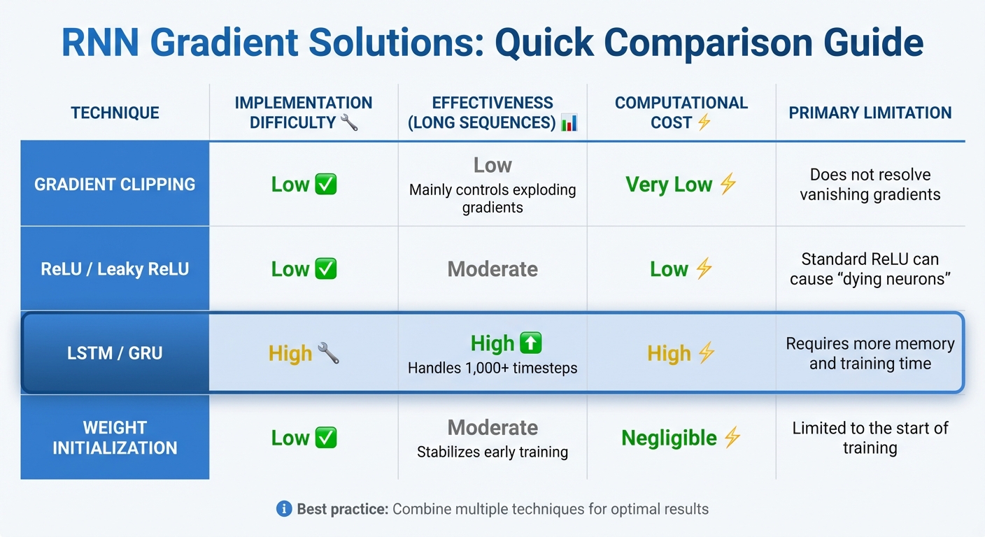
| Technique | Implementation Difficulty | Effectiveness (Long Sequences) | Computational Cost | Primary Limitation |
|---|---|---|---|---|
| Gradient Clipping | Low | Low (mainly controls exploding gradients) | Very Low | Does not resolve vanishing gradients |
| ReLU / Leaky ReLU | Low | Moderate | Low | Standard ReLU can cause "dying neurons" |
| LSTM / GRU | High | High (handles 1,000+ timesteps) | High | Requires more memory and training time |
| Weight Initialization | Low | Moderate (stabilizes early training) | Negligible | Limited to the start of training |
In practice, these methods are often combined for optimal results. For instance, proper weight initialization ensures stable early training, gradient clipping prevents exploding gradients, and LSTMs are used to capture long-term dependencies effectively.
Conclusion
Vanishing gradients arise due to issues like saturating activation functions, repeated multiplications in recurrent layers, and improper weight initialization. As gradients diminish exponentially over time, the network struggles to capture long-range dependencies, often stalling or slowing down the learning process.
The best solution depends on the task at hand. For scenarios requiring long-term memory - such as analyzing entire paragraphs or time series data exceeding 100 timesteps - architectures like LSTMs and GRUs are highly effective. Their gated mechanisms help maintain gradient flow over extended sequences. On the other hand, for shorter sequences (10–20 timesteps) or extremely deep networks, switching from Sigmoid or Tanh to non-saturating activation functions like ReLU or LeakyReLU can provide a straightforward solution.
Using proper weight initialization methods, such as He or Xavier initialization, ensures gradients remain stable from the outset. Gradient clipping is another valuable tool, as it prevents gradients from exploding and causing instability.
FAQs
How do LSTMs address the vanishing gradient problem in traditional RNNs?
LSTMs address the vanishing gradient problem that often plagues traditional RNNs with an architecture designed to handle gradients more effectively over time. In standard RNNs, gradients are repeatedly multiplied by the same weight matrix during backpropagation. When the eigenvalues of this matrix are smaller than 1, the gradients shrink exponentially, making it nearly impossible for the network to capture long-term dependencies.
What sets LSTMs apart is their gated memory cell structure. Instead of depending solely on multiplicative updates, LSTMs incorporate additive connections in their cell state, which helps maintain gradient stability. The forget, input, and output gates work together to dynamically decide which information to keep, update, or discard. This mechanism significantly reduces the issue of gradient decay, allowing LSTMs to recognize and learn patterns over much longer sequences than traditional RNNs can manage.
How does weight initialization impact RNN performance?
Weight initialization is a critical factor in how well recurrent neural networks (RNNs) perform. Since the same weight matrix is applied at every time step, a poor starting point can make training unstable. If the weights are too small, gradients shrink exponentially, leading to the vanishing gradient problem. On the flip side, if the weights are too large, gradients can grow uncontrollably, causing the model to become unstable.
To address these challenges, modern initialization techniques have been developed. For example, Xavier/Glorot initialization works well with sigmoid or tanh activations, while He initialization is better suited for ReLU activations. These methods adjust the scale of weights based on the layer size and activation function, ensuring gradients remain stable during training. Specifically for RNNs, orthogonal or unit-norm initializations are highly effective. They help maintain the length of hidden states over time, which minimizes gradient-related issues. Pairing these approaches with methods like gradient clipping can further stabilize training, even when working with long sequences.
Why are ReLU and Leaky ReLU often better than sigmoid and tanh for some RNN tasks?
ReLU and Leaky ReLU are often chosen over sigmoid and tanh for specific RNN tasks because they tackle the vanishing gradient problem more effectively. Sigmoid and tanh functions compress values into smaller ranges, which can cause gradients to diminish during backpropagation. In contrast, ReLU and its variants maintain more stable gradients by avoiding rapid saturation.
Another advantage is their computational efficiency, which can accelerate training. Since they handle larger input values without saturating, ReLU and Leaky ReLU are especially useful for deep networks or tasks involving long-term dependencies.