
GRU Hyperparameter Tuning: Study Summary
If you want a short answer: start with Adam or AdamW, a peak learning rate around 6e-4 to 1e-3, warmup plus cosine decay, and global norm clipping at 1.0. That mix shows up again and again across GRU studies.
I’d treat the tuning order like this:
- Optimizer: Adam or AdamW
- Learning rate: 0.0006 to 0.001 at peak
- Schedule: linear warmup, then cosine decay
- Gradient clipping: global norm at 1.0
- Weight decay: around 0.1 on weights and embeddings only
- Dropout: 0.0 to 0.2, often higher on smaller datasets
- Model size: start shallow; add layers only if the dataset is big enough
- Window size: test a few sequence lengths instead of defaulting to the largest
- Batch size: fit VRAM first; use gradient accumulation if needed
- Stopping: save the best validation-loss checkpoint and stop early when loss stalls
A few numbers stand out. Studies often use validation checks every 250 to 2,000 iterations. Single-layer GRUs with 64 to 256 hidden units are a common starting point on smaller datasets. And one result found that clipping at 1.0, with tuned momentum, closed 96% of the gap between SGD and Adam in a 160M-parameter model.
My main takeaway is simple: don’t over-tune everything at once. I’d lock in a stable optimizer and schedule first, use clipping as a safety check, keep the model small at the start, and let validation loss decide whether more context, depth, or batch size is worth it.
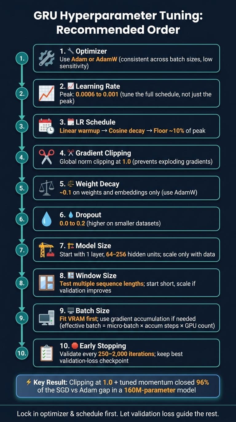
GRU Hyperparameter Tuning Order: Step-by-Step Cheat Sheet
Optimizer and Learning-Rate Findings
Optimizer choice and learning rate are two settings researchers tune again and again in GRU work. Get either one wrong, and even a well-built model can have a hard time converging in a steady way.
Why Adam Shows Up So Often in GRU Studies
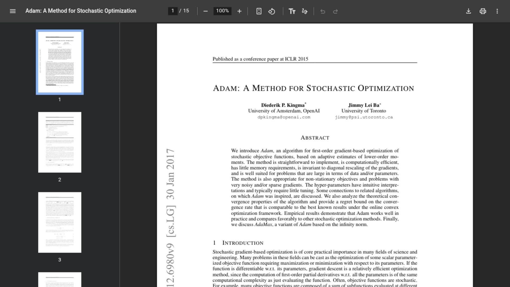
Adam keeps showing up as the default for GRU training because it deals with uneven gradients better than SGD.
SGD can narrow the gap in small-batch training, but it usually takes more steps and more careful tuning. In practice, the difference is pretty clear: Adam stays steady across batch sizes, while SGD tends to fall off as batch size grows.
Recent work points to a handy shortcut for Adam in sequence tasks too. Setting the momentum terms to the same value (β1 = β2), often 0.95, can keep performance near the best range while making tuning simpler.
| Optimizer | Sequence Task Performance | Batch Size Sensitivity | Notes |
|---|---|---|---|
| Adam / AdamW | High (baseline) | Low | Consistent across scales |
| SGD + Momentum | Low to moderate | High | Needs small batches and heavy tuning to compete |
So the optimizer matters, but the step size and the schedule around it matter just as much.
Low Learning Rates and Scheduled Decay Patterns
Across studies, the same pattern shows up: a low peak learning rate combined with warmup and decay. A common setup is linear warmup followed by cosine decay, with a low floor near 10% of the peak rate.
That pattern keeps turning up in sequence tasks because it helps steady gradient estimates early in training, then gradually lowers the rate toward its minimum. Put simply, don't tune the peak rate by itself. Tune the whole schedule.
Once the step size is in place, gradient clipping becomes the next lever to watch.
sbb-itb-903b5f2
Gradient Stability and Clipping
Once the learning rate is in place, clipping becomes the main safety check for long sequences, noisy updates, and large batches. The practical question is simple: which clip value works most often, and which clipping mode do people usually use?
Typical Clipping Ranges and When They Matter
A clipping threshold of 1.0 is the most common default in modern sequence modeling setups. In most cases, that means using global norm clipping, which caps the gradient L2 norm before the optimizer step.
Large batches tend to need clipping more often, and 1.0 is the standard place to start. Without clipping, large-batch training can diverge. Small batches can sometimes train fine without it, but 1.0 is still a safe default. If clipping kicks in a lot, that's often a sign the learning rate or batch size is off.
Here’s the main clipping mode that shows up in practice:
| Clipping Method | Purpose | Typical Trigger | Reported Effect |
|---|---|---|---|
| Global Norm Clipping (Gclip) | Prevents exploding gradients and unstable updates | L2 norm exceeds the threshold, usually 1.0 | Improves training reliability and helps prevent divergence in large batches |
So clipping is best viewed as a stability control. It helps keep training on the rails, but it won’t rescue a bad learning rate.
What Clipping Fixes and What It Does Not
Clipping reliably cuts down exploding gradients, sudden loss spikes, and NaN updates, but it does not fix slow convergence or overfitting. It also should not be treated as a substitute for choosing a sound learning rate or a sensible batch size.
One result stands out. In a 160M-parameter model, a clipping threshold of 1.0, paired with optimal momentum, helped close 96% of the performance gap between SGD and Adam.
Clipping also does not solve vanishing gradients. In GRUs, that job is handled by the gating architecture. If training still diverges with clipping enabled at 1.0, the next places to look are the learning rate and the initialization range.
And if clipping still isn’t enough to calm things down, the next levers to tune are initialization and network size.
Initialization and Network Size
Now the question shifts from what the model does to how big it should be and how to set it up at the start. A good rule of thumb: begin with a shallow model unless the task clearly calls for more depth.
Single-Layer vs. Deeper GRU Configurations
With small datasets, shallow GRU setups are usually the safer bet. Adding more layers can push overfitting risk up fast. Put simply, model depth should match the amount of data you have.
Here’s a simple way to think about it:
| Configuration | Layer Depth | Hidden Units | Dataset Size / Use Case |
|---|---|---|---|
| Single-Layer | 1 layer | 64–256 units | Small datasets, high overfitting risk; safest starting point |
| Shallow Multi-Layer | 2–3 layers | 256–512 units | Moderate datasets; test carefully for overfitting before adding depth |
| Deeper Stack | 4+ layers | 512+ units | Large datasets only; overfitting risk rises sharply without sufficient data |
That pattern is pretty common in practice. If your dataset is limited, a single-layer GRU often gives you the best shot at stable training without piling on extra risk. As data volume grows, adding a bit more depth can make sense. But going deep too early is often where things start to go sideways.
Once depth is chosen, the next step is weight initialization.
Initialization Ranges in Search-Based Tuning
Search ranges should be used to test model capacity, not to patch unstable training.
For brand-new GRUs, use random initialization. If you’re fine-tuning, start from checkpoints instead. When teams search for the right number of hidden units and the right dropout rate, they usually set discrete ranges first and then run grid search, random search, or Bayesian optimization across those options.
Batch size is usually less about theory and more about hardware limits. In most cases, it’s capped by the GPU memory you have available.
After model size is locked in, sequence window length becomes the next big lever to tune.
Sequence Handling, Training Setup, and Final Summary
The remaining tuning choices mostly come down to two things: how much context the GRU can look at and how you run training without wasting time or memory.
Optimal Window Size Is Usually Task-Specific
Once you've worked through the optimizer, gradient clipping, and model size, the next lever is context length. In the sequence studies summarized here, the context window (block_size) is task-specific, not one-size-fits-all.
That means researchers usually test a handful of sequence lengths instead of just picking the biggest one and hoping for the best. A short window is often the smart place to begin, especially for debugging. Then, if validation shows the task needs more context, increase it step by step.
Batch Size, Epoch Limits, and Validation-Based Stopping
After context length, the next issue is simple: can the data fit into memory? If VRAM is tight, gradient accumulation helps increase the effective batch size without forcing a larger micro-batch onto the GPU.
Effective batch size = micro-batch size × accumulation steps × GPU count.
For training duration, many studies use a max-iteration limit instead of a fixed epoch count. That gives tighter control on large datasets. Validation loss is checked at set intervals, often every 250 to 2,000 iterations, and the score is averaged across multiple validation batches. In practice, teams usually keep only the checkpoint with the best validation loss.
Key Research Patterns: A Final Recap
Put together, the studies suggest a clear tuning order: pick the right context length, make the batch fit memory, and control training with validation.
| Configuration | Window Size | Effective Batch Size |
|---|---|---|
| Debug / Small | Short (e.g., 256 tokens) | Small (e.g., ~16,384 tokens/iter) |
| Fine-tuning | Task-specific (often 1,024 tokens or the task maximum) | Task-dependent |
| Long-Context | Large (e.g., 1,024 tokens) | Large (e.g., ~491,520+ tokens/iter) |
Use the smallest window that still covers the task's dependencies, then scale up only if validation gets better.
FAQs
How do I tune GRU hyperparameters in the right order?
Start with a simple baseline: turn dropout off. Then tune things in this order:
- dropout rate
- weight decay with AdamW
- gradient clipping
- learning-rate schedule
For smaller datasets, use a small nonzero dropout. For weight decay, start at 0.1. Clip gradients at 1.0. For the learning rate, use a cosine schedule with linear warmup.
If you're using AdamW, apply weight decay only to weights and embeddings. Don’t apply it to biases or normalization terms.
When should I increase GRU depth or hidden size?
Increase GRU hidden size when your task involves complex patterns or long sequences that need more room for the model to store and process information.
A larger hidden size lets the model learn more detailed relationships. The trade-off is simple: it also uses more memory and takes longer to train. So there’s a balance here between model capacity and the compute you have on hand.
How do I know if my window size is too large?
Common signs include worse performance, poor memory use, and unstable training. With GRUs, a window that’s too large can stop helping after a point. Instead, it can make gradient flow harder to keep in check, which increases the risk of vanishing or exploding gradients.
It also helps to watch loss convergence and output quality. If training gets less stable, or the model starts losing context and generating repetitive, looping text, the window size may be too large.